Biological systems are usually much too complicated to be understood in their entirety. Scientific progress is therefore generally based on the fragmentation of the systems under investigation. This means the system is broken down into smaller parts or subsystems, which can then be more easily approached. However, such a reduction to a lower level - for instance - from behavior to reflexes, from reflexes to neuronal cells, or from cells to molecules - also has serious shortcomings. First, the overview of the whole system may be lost. Looking at the lower level, one may not see "the forest for the trees" because many system properties are only understandable when not only the individual parts of the system, but also the cooperation of these parts are taken into account. Second, this reduction may further increase the gap that already exists between biological research and the investigation of problems on more complex levels, such as those considered in psychology or even philosophy. To make this gap smaller "holistic" approaches are required.
One sensible way to oppose this reductionistic path is the use of simulation. The construction of quantitative models, usually in the form of computer simulation, is an important tool in biology. Such a simulation allows a step in the other, "antireductionistic" direction, namely to construct complex systems from smaller, simple elements. Through investigation of the simulated system, the properties of the whole system can be better understood.
The tool of simulation is particularly important for understanding the dynamic properties of systems. Such dynamic properties are often produced by feedback loops within the system. However, the human brain does not seem very well adapted to grasp such systems. Simulations could improve this situation. We might become more familiar with the properties of dynamic systems and thus train ourselves to understand such systems so that, even without an explicit computer simulation, some predictions could be made. Such dynamic systems occur in many fields, from genetics, metabolism, and ecology to, of course, neurobiology and ethology . Although this book will concentrate on the latter two, the tools provided can also be applied to the other fields. But these tools are also applicable to fields outside biology, e. g., psychology, and to even more distant areas, such as economics, physics, and electrotechnology (which in fact gave rise to many of these ideas).
Ethology, although an important field in biology, had been attracting less interest in recent decades mainly because of a lack of theoretical concepts. This has, however, dramatically changed in recent years because the emergence of the theory of artificial neural networks (ANN) and the field of artificial life, has led to the development of a great number of models and modeling tools that can now be fruitfully applied to ethology and neuroethology. Although the treatment of simple neuronal models was already an important subject of early biological cybernetics, the focus of interest later moved to "pure" systems theory. Only in the last decade did the field of ANN approach gain its enormous thrust. These two fields have not yet been brought into intensive contact with each other, but the consideration of dynamic properties so central to systems theory has the potential to make a great impact on ANN. This book attempts to combine both approaches which, as mentioned, stem from the same roots. It can be expected that both fields will profit from each other.
Usually textbooks on these fields are loaded down with a great deal of mathematics, which makes them somewhat indigestible for the typical student of biology. To minimize these problems, this book tries to avoid the use of mathematical formulas as far as possible. The text is based not on differential equations or on complex variables, but rather on illustrations. It nevertheless provides sufficient information to permit the reader to develop quantitative models. Technical aspects are relegated to the appendices.
The first part of this book is based on an earlier version of my book "Biologische Kybernetik", which was inspired by the exciting lectures of D. Varju at the University of Tübingen. Writing this greatly expanded version of the book would not have been possible without the help of a number of colleagues who met in a research group funded by the Center of Interdisciplinary Research (ZiF) of the University of Bielefeld. I mainly want to thank to H. U. Bauer, Frankfurt; H. Braun, Karlsruhe; G. Hartmann, Paderborn; J. Dean, A. Dress, P Lanz, H. Ritter and J. Schmitz, all from Bielefeld; and H. Scharstein, Cologne, for a number of helpful comments. Furthermore, l would like to thank to A. Baker who helped with the English in an earlier version of the manuscript, A. Exter for the preparation of many figures, and P. Sirocka and Th. Kindermann for providing Figures B 5.3 and B 5.1, respectively. Furthermore, I owe a debt of gratitude to many students of my lectures who succeeded in finding errors and unclear formulations in the text. Of course, the responsibility for all remaining flaws is my own.
April 1996 Holk Cruse
Ten years ago, the first edition of the book ”Neural Networks as Cybernetics Systems“ has been published by Thieme. At this time there was still an ongoing debate whether the neural network approach comprises just a fashionable, but short living hype. Meanwhile this approach is well established. Understanding complex systems by means of simulation is more and more accepted, also within biology. The more it is important to provide students with a tool that helps to understand and also actively perform simulations. This is particularly important for students their primary education was not in mathematics or in computer science. It is the goal of this text to provide such a tool. In the first part, both linear and nonlinear aspects of systems theory, sometimes called filter theory or theory of dynamical systems, are treated in a way that mathematical terms are avoided as far as possible. In part II this is extended to the theory of massively parallel systems, or theory of neural networks. This qualitative approach is also suited as a first step for students that later plan to follow a more thorough quantitative understanding.
Appearing as an (open access) e-version, the handling of the text is easier compared to the earlier printed version, figures are coloured, errors are corrected, (hopefully new errors appear at a minimum), and some chapters, in particular those concerning the important field of recurrent networks, are added anew. The most helpful extension however concerns the software package that allows to perform exercises concerning simulations for part I. This package is written so that it can be used in an extremely simple way. Extensions for part II are in preparation.
January 2006 Holk Cruse
Up to now, using the systems theory approach, we have dealt with systems where the number of parallel channels is very small. Most systems possess one or two parallel channels. This highest value, i. e., four, occurred in an example illustrated above (Fig. 8.14), if the feedback channels running in the opposite direction are included. Many systems, especially nervous systems, are endowed with structures containing an abundance of parallel channels. This is particularly clear for the above example where typically each muscle is excited by a large number of α- and of γ-motorneurones on the efferent side and by many sensory neurons (e. g., muscle spindles), on the afferent side. In previous considerations, models were constructed on the assumption that it is useful to simplify the systems by condensing a great number of channels to just a few. However, some characteristics of these systems become apparent only when the highly parallel or, as they are often called, massively parallel structure is actually considered. More recently such systems have been called neuronal nets or connectionist systems, but they had already been investigated in the early days of cybernetics ( Reichardt and Mac Ginitie 1962 , Rosenblatt 1958 , Steinbuch 1961 , Varju 1962 , 1965 ).
In order to make it possible to deal with a large number of parallel connections, we introduce a new basic element which, in the present context, we will call a neuroid, to show its difference from real neurons. The neuroid is a purely static element. Effects such as dynamic effects, for example low-pass properties (see Part I - Chapter 4 ) as well as more complicated properties such as spatial summation, or spatial or temporal potentiation, are not considered in this simple form of a neuroid. Artificial neuronal nets consist of a combination of many of these basic elements. The neuroid displays the following basic structures (Fig. 9.1 a, b). It has an input section which receives signals from an unspecified number of input channels and summates them linearly. In principle, this input section may correspond to the dendritic section of a classic neuron, though it should be noted that there are important differences, as mentioned above. The input section of a neuroid acts as a simple summation element. It is represented in Figure 9.1 in two different ways. In Figure 9.1 a it corresponds to the usual symbol for the summation. In Figure 9.1 b the input section is represented by a broad "column." This has advantages for subsequent figures, but should not encourage the (unintended) interpretation that this represents a real dendritic tree with the dynamic properties mentioned above.
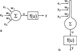
Fig. 9.1 Two schematic presentations of a neuroid. In this example the neuroid receives three input values x1, x2, x3. Each input is multiplied by its weight w1, w2, and w3, respectively. The linear sum of these products, u, is given to an, often nonlinear, activation function f(u) which provides the output value y. (a) resembles more the morphology of an biological neuron, (b) permits an clearer illustration of the connections and the weights
The inputs impact on the neuroid via "synapses." At these synapses the incoming signals may be subject to different amplification factors or weights which are referred to by the letter w. Generally, these weights may adopt arbitrary real values. Positive weights may formally correspond to an excitatory synapse, a negative weight to an inhibitory synapse. After multiplication with their corresponding weights w1, w2, and w3, the incoming signals x1, x2, and x3 are summated as follows:
 .
.
This value is eventually transformed by a static characteristic of a linear or, in most cases, nonlinear form which is often called the activation function. Two kinds of nonlinear characteristics are normally used in this context, namely the Heaviside (all-or-nothing) characteristic (Fig. 5.12) and the sigmoid characteristic. The logistic function already mentioned 1/(1 + e-ax) is frequently used as a sigmoid characteristic (Fig. 5.11). If the activation function is referred to by f(u), the resultant output value of the neuroid is y = f(Σ xiwi).
The neuroids can be linked together in different ways. The so-called feedforward connection is the one that can be most easily understood. The neuroids are grouped on two levels or layers, the input layer and the output layer (Fig. 9.2a). Each of the n neuroids of the input layer has only one input channel xi which receives signals from the exterior world. The outputs of the neuroids of the first layer may be connected with the inputs of all m neuroids of the second layer. In this way, one obtains mn connections. Although the arrangement of Figure 9.2a does correspond more to biological structure, the matrix arrangement (Fig. 9.2b) is useful in providing an easily understood representation. Here the individual weights can be written as a matrix in a corresponding way. The connection between the j-th neuroid of the first layer and the i-th neuroid of the second is assigned the weight wij. The output of the i-th neuroid of layer two can thus be calculated as yi = fi(jΣ wij xj). Using the feedforward connection, an unlimited number of additional layers may be added. Figure 9.3 a, b shows a case with three layers. Since the state of those neuroids which belong neither to the top nor the bottom layers is, in principle, not known to the observer, these layers are called hidden layers. It is also possible, of course, that direct links exist between nonadjacent layers.
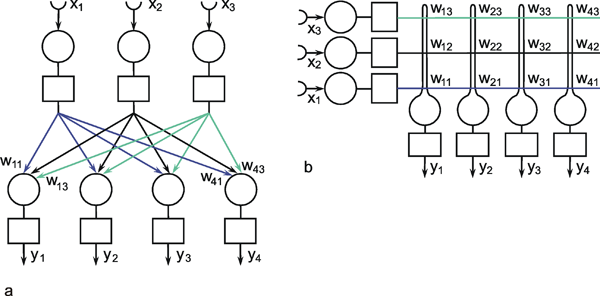
Fig. 9.2 A two-layer feedforward network with n (= 3) units in the input layer and m (= 4) output units in the output layer. xi represent the input values, yi the output values. The weights wij have two indices, the first corresponds to the output unit, the second to the input unit. As in Fig. 9.1, (a) more resembles the arrangement of a net of biological neurons, whereas the matrix arrangement of (b) permits a clearer illustration of the connections and the weights (only some weights are shown in (a)). The boxes represent unspecified activation functions
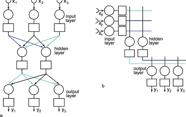
Fig. 9.3 A three-layer feedforward network with three input units, two units in the intermediate, "hidden" layer, and three output units. The boxes represent unspecified activation functions. Again, the illustration in (a) more resembles the biological situation, and the matrix arrangement provides an easier overview, particularly, if in addition direct connections between input and output layer are used (not shown)
Another form of connection occurs in the form of so-called recurrent nets. These contain feedback channels as described earlier for the special case of the feedback controller. In its simplest form, such a net consists of one layer. Each neuroid is provided with an input xi from the exterior world and also emits an output signal yi. At the same time, however, these output signals are relayed back to the input level, as shown in Figure 9.4a. Here, too, the matrix arrangement is helpful in illustrating this more clearly (Fig. 9.4b). The output of the j-th neuroid can, in principle, be calculated in the same way, namely as yi = fi(jΣwij yj), with neuroids i and j belonging the same layer, of course. From studies of the stability of feedback systems ( Part I - Chapter 8.6 ) it follows that the behavior of recurrent nets is generally much more complicated than that of feedforward nets. It should, however, be emphasized that both these types of nets are not alternatives in a logical sense. In fact, the recurrent net represents the general form since, by an elimination of specific links (i. e. introducing zero values for the corresponding weights), it can immediately be transformed into a feedforward net including feedforward nets of several layers (Fig. 9.5). For this purpose most of the weights (Fig. 9.4) have to become zero.
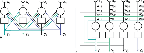
Fig. 9.4 A recurrent network with four units. In the case of the recurrent network the arrangement resembling biological morphology (a) is even less comfortable to read compared to the matrix arrangement (b). xi represent the input values, yi the output values. The boxes represent unspecified activation functions
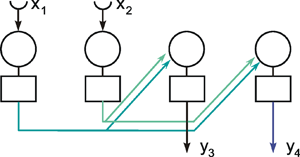
Fig. 9.5 When some selected weights of the network shown in Fig. 9.4 are set to zero, a feedforward net, in this example with two layers, can be obtained. To show this more clearly, the connections with zero weights are omitted in this figure. xi represent the input values, yi the output values
The properties of a net are determined by the types of existing connections as well as by the values taken by the individual weights. To begin with, the properties of nets with given weights will be discussed. Only later will we deal with the aspect to how to find weights, by searching for a net with desired transfer properties. These procedures are often called "learning."
The designation of elements of these nets as neuroids suggests their interpretations as neurons. It should be mentioned, however, that other interpretations are conceivable as well, for example, in terms of cells which, during the development of an animal, mutually influence each other, e. g., by way of chemical messenger substances (see Chapter 11.1 ), and form specific patterns in the process. In a similar way, growing plants might influence each other and thus the whole plant might be represented by one "neuroid:" Another example are genes of a genom which may influence each other's activity by means of regulatory proteins.
Artificial neuroids have a number of inputs xi and one output y. The input values are multiplied by weights wi. The linear sum u might be subject to a (nonlinear) characteristic f(u). Dynamic properties like temporal low-pass filtering, or temporal and spatial summation are ignored. The neuroids might be arranged in different layers, an input layer, an output layer and several hidden layers. The neuroids might be connected in a pure feedforward manner or via recurrent connections.
In the first four sections of this chapter, networks will be considered that are repetitively organized. This means that all neuroids have the same connections with their neighbors. In the subsequent three sections feedforward nets with irregular weight distribution, will be dealt with.
A simple structure, realized in many neuronal systems, is the so-called divergence or fan-out connection. Figure 10.1 shows a simplified version. In this case, the two-layer feedforward net contains the same number of neuroids in each layer. Each neuroid of the second layer is assigned an input from the neuroid directly above it as well as inputs with smaller weights from the two neighboring neuroids. In a more elaborate version of this system, a second layer neuroid would be connected not only with its direct first layer neighbor but also with neuroids that are further removed; in this case, the value of the weights, i. e., the local amplification factors, are usually reduced as the distance increases. (By maintaining the sum of all the weights of a neuroid equal to one, the amplification of the total system also retains the factor one.) Figure 10.2a shows the response of such a system when one neuroid at the input is given the input value 1, while all others are given the value 0. For this input function, the output shows an excitation that corresponds directly to the distribution of individual weights. Since the input function can be considered an impulse function in spatial rather than in temporal domain, this response of the system can accordingly be defined as weighting function. This function directly reflects the spatial distribution of the weights. Figure 10.2b shows the response of the same system to a spatial step function. Here the neuroids 1 to i of the input layer are given the excitation 0, and the subsequent neuroids i + 1 to n, the excitation 1. In the step response the edges of the input function are rounded off. Qualitatively, then, the system acts like a (spatial) low-pass filter. In contrast to the step response of a low-pass filter in the temporal domain, both edges of the step are rounded off in a symmetrical way. This property is already reflected in the symmetrical form of the weighting function (see difference to Figure 4.1). This property also affects the phase frequency plot, not shown here, which shows a phase shift of zero for all (spatial) frequencies. In a qualitatively similar way as described for the temporal low-pass filter, the corner frequency of the spatial low-pass filter is the lower the broader is the form of the weighting function. It should be mentioned that the Fourier analysis can, of course, also be applied to spatial functions. In Figure 3.1 this could be done by interpreting the abscissa as a spatial axis instead of a temporal one. The rectangular function therefore corresponds to a regularly striped pattern. Examples of spatial sine functions will be shown in Box 4 .

Fig. 10.1 A two-layer feedforward net with the same number of input and output units. Only a section of the net is illustrated. Directly corresponding neuroids in the two layers are connected by a weight of 0.5, the two next neighbors by weights of 0.25. This is indicated by large and small arrowheads, respectively. (b) shows the weights of the neuroids arranged in the matrix form described earlier
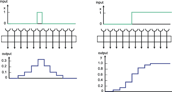
Fig. 10.2 Impulse response (a) and step response (b) of a two-layer feedforward network (spatial low-pass filter) as shown in Fig. 10.1, but with lateral connections including three neighbors instead of only one. The network is shown as a box. The central weight is 0.3. The weight values decrease symmetrically to right and left, showing values of 0.2, 0.1, and 0.05, respectively. These values can be directly read off the output, when a "spatial impulse" (a) is given as input, i. e., only one unit is stimulated by a unity excitation. The step response (b) is symmetrically, too, and represents the superposition of the direct and lateral influences. Input (x) and output (y) functions are shown graphically above and below the net, respectively
A spatial low-pass filter could be interpreted as a system with the property of "coarse coding." At first sight, the discrete nature of the neuronal arrangement might lead to the assumption that spatial resolution of information transfer is determined by the grid distance of the neurons. This seems to be even more the case when the neurons have broad and overlapping input fields. This overlap is particularly obvious for sensory neurons. For example, a single sensory cell in the cochlea is not only stimulated by a tone for a single frequency, but by a very broad range of neighboring frequencies. However, the sensitivity of the cell decreases with the distance between stimulating frequency and best frequency. In turn, this means, that a single frequency stimulates a considerable number of neighboring sensory cells. A corresponding situation occurs, if we consider several layers of neurons with fan-in fan-out connections as shown in Figure 9.3. The units in the second layer receive input also from neighboring units. In this way, as already mentioned, the exactness of the input signal degrades, and one might conclude that capability to determine the spatial position of a stimulus might grow worse as the grid size of the units increases. However, it could be shown ( Baldi and Heiligenberg 1988 , Rumelhart and McClelland 1986 ) that determination of the position of a single stimulus is better, the more the input ranges between neighboring units overlap. If, for instance, a single stimulus is positioned between two sensory units, the ratio of excitation of these two sensory units depends on the exact position of the stimulus relative to the two units. Thus, the information on the exact position is still contained in the system. An obvious example is represented by the human color recognition system. We have only three types of sensory units, but can distinguish a high number of different colors. These are represented by the ratios of excitation of these three units. Thus, although the system morphologically permits only "coarse coding," the information can be transmitted with a much finer grain by means of parallel distributed computation. Furthermore, such a spatial low-pass filter is more tolerant of failure of an individual unit, the more the input fields on the neighboring units in the net overlap.
Networks with excitatory fan-out connections show low-pass properties in the spatial domain. Symmetrical connections provide low-pass filters with zero phase shifts. In spite of coarse coding, in such a distributed network information can be transmitted with a much finer grain than that given by the spatial resolution of the grid.
Figure 10.3 shows a simple net with the same connection pattern as Figure 10.1, but a different distribution of weights. Each neuroid of the second layer receives an excitation, which has been given the weight 1, from the neuroid located directly above. From the neighboring neuroids of the first layer it additionally receives inputs of negative weights. As above, the figure shows only the linkages with the nearest neighbors; but linkages with neuroids further away, whose weights decrease correspondingly, are possible. In this case, the sum of all weights of a neuroid should be zero. Figure 10.4a shows the impulse response, i. e., the weighting function of the system when the connections with non-zero weights reach up to three neuroids in either direction. Correspondingly, Figure 10.4b shows the response to the step function. A comparison with the time filters shows that this system is endowed with high-pass properties. Here, too, the response, in contrast to the response of the time filter, exhibits symmetrical properties. These are reflected in the form of the step response and of the impulse response (compare to Figure 4.3). The fact that in this net the lateral neighbors exhibit negative weights is called lateral inhibition in biological terms. This is a type of connection which can be found in many sensory areas. By means of such a network, a low contrast in the input pattern can be increased. For example in the visual system such a low level contrast could result from using a low quality optical lens. An appropriate lateral inhibition could cancel this effect. A pure high-pass filter transmits only changes in the input pattern and thus produces an output which is independent of an absolute value of the input intensity. Thus, the output pattern is independent of the mean value of the input signals. There are also other forms of lateral inhibition which use recurrent connections (see Varju 1962 , 1965 ).

Fig. 10.3 A section of a two-layer feedforward network as shown in Fig. 10.1, but with a different weight distribution. Now, two directly corresponding neuroids in the two layers are connected by a weight of 1. The weights of the connections to the two neighboring units (thin arrows) are -0.5, forming the so-called lateral inhibition. (b) shows the corresponding matrix arrangement of the weights (see Fig. 9.2b)
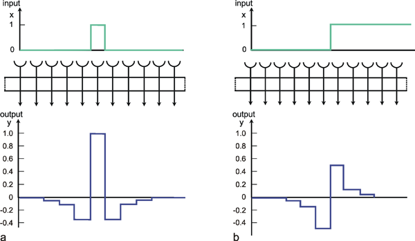
Fig. 10.4 Impulse response (a) and step response (b) of a two-layer feedforward network as shown in Fig. 10.3, but with lateral connections including three neighbors instead of only one (spatial high-pass filter). The network is shown as a box. The central weight is 1. The weight values decrease symmetrically to right and left, showing values of -0.35, -0.1, and -0.05, respectively. These values can be directly read off the output, when a "spatial impulse" (a) is given as input, i. e., only one unit is stimulated by a unity excitation. Input (x) and output (y) functions are shown graphically above and below the net, respectively
Networks showing connections with lateral inhibition can be described as a spatial high-pass filter.
In contrast to the time filters, a spatial band-pass filter can be obtained by connecting a spatial low-pass filter and a spatial high-pass filter in parallel. This occurs in many sensory areas, such as for example in the retina of mammals. As long as there are no nonlinearities, the weighting functions can be added up such that still only two layers are necessary. Figure 10.5a shows the weighting functions of a low-pass filter (E), a high-pass filter (I), and the sum of both (RF), plotted as a continuous function for the sake of simplicity. For the pure band-pass filter the sum of all weights acting on one neuron should accordingly be of value 1 (if this sum is larger than 1, we obtain a spatial lead-lag system, see Fig. 4.10). In this case the positive connection described for the high-pass filter is not more necessary, because this effect is provided by the positive low-pass connection. If we extend the one-dimensional arrangement of neuroids to a two-dimensional arrangement, making the corresponding connections in all directions, Figure 10.5a can be considered as the cross section of a rotation-symmetrical weighting function (Fig. 10.5b). When, as is the case in Figure 10.5, the weighting function of the high-pass filter is wider, but has smaller weights than that of the low-pass filter, the result will be a weighting function with an excitatory center and inhibitory surrounding neighborhood. This connectivity arrangement is also known as "Mexican hat." This constitutes a representation of simple receptive fields as found in the visual system. When the weighting function of the low-pass filter is wider, but has smaller weights than the high-pass filter, we obtain a receptive field with a negative "inhibitory" center and a positive, excitatory surrounding.
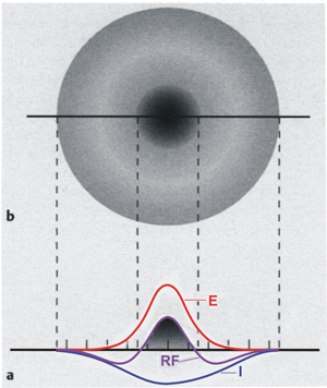
Fig. 10.5 Distribution of the weights on a twodimensional, two-layer feedforward network. (a) shows a cross section similar to those presented in Figs. 10.2a (E) and 10.4a (I), but for convenience the weighting functions are shown in a continuous form rather than in discrete steps. An excitatory center (dark shading) and an inhibitory surrounding is produced when both weighting functions are superimposed, forming a receptive field (RF). (b) shows this receptive field in a top view
It should be mentioned that in an actual neurophysiological experiment one usually investigates the weighting function, not by presenting an impulse-like input and measuring all the outputs values of the neurons in the second layer, but by recording from only one neuron of the second layer and moving the position of the impulse along the input layer.
Circular receptive fields with excitatory centers and inhibitory surroundings form the elements of a spatial band-pass filter.
Spatial Filters in the Mammalian Visual System
A simple, qualitative experiment can illustrate that the human visual system shows band-pass properties. In Figure B4.1 the abscissa shows spatial sinusoidal waves of increasing frequency. Along the ordinate the amplitude of these sine waves decreases. In this way, the figure can be considered as illustrating the amplitude frequency plot. The sensitivity of the system, which in the usual amplitude frequency plot is shown by the gain of the system, is demonstrated here in an indirect way. Instead of using the gain, the sensitivity is shown by regarding the threshold at which the different sine waves can be resolved by the human eye. The line connecting these thresholds is illustrated in Figure B4.1 b. It qualitatively follows the course of the amplitude frequency plot of a band-pass filter.
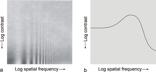
Fig. B 4.1 Qualitative demonstration of the low-pass properties of the human visual system. As in the amplitude frequency plot, on the abscissa, sine waves with logarithmically increasing spatial frequency are plotted. The contrast intensity of each sine wave decreases along the ordinate. The subjective threshold, which is approximately delineated in (b), follows the form of the amplitude frequency plot of a low-pass filter ( Ratliff 1965 )
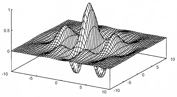
Fig. B 4.2 A Gabor wavelet is constructed by first multiplying two cosine functions, one for each axis, which in general have different frequencies. This product is then multiplied by a two-dimensional Gaussian function
Electrophysiological recording in the cortex of the cat indicate that the "Mexican hat" is only a first approximation for the weighting function of the spatial filter ( Daugman 1980 , 1988 ). The results could be better described by so-called Gabor wavelets. These are sine (or cosine) functions multiplied by a Gaussian function. In a two-dimensional case, the frequency of the sine wave might be different in the two directions. An example is shown in Figure B4.2. The application of Gabor wavelets to transmission of spatially distributed information could be interpreted as a combination of a strictly pixel-based system and a system which performs a Fourier decomposition and transmits only the Fourier coefficients. The former system corresponds to a feedforward system with no lateral connections. It provides information about the exact position of a stimulus but no information concerning the global coherence between spatially distributed stimuli. Conversely, a Fourier decomposition provides only information describing the coherence within the complete stimulus pattern but no direct information about the exact position of the individual stimulus pixels. When a superposition of Gabor wavelets with different sine frequencies is used (for example a sum of wavelets, the frequency of which is doubled for each element added), they represent a kind of local Fourier decomposition, i. e., provide information on the coherence in a small neighborhood, but also contain spatial information. Thus, there is a trade-off between spatial information, i. e., local exactness, and information on global coherence.
A Gabor wavelet could be constructed by several ring-like zones of excitatory and inhibitory lateral connections. Thus, the "Mexican hat" can be considered as an approximation to a Gabor wavelet the sine frequency of which is chosen such that the second maximum of the sine wave, i. e., the first excitatory ring, is far enough distant from the center of the Gaussian function that its contribution can be neglected.
The following network has a similar structure to the inhibitory net described above. Each neuroid of the second layer obtains a positive input from the neuroid directly above it, which has been assigned the weight 1. All other neuroids obtain a negative, i. e., inhibitory, influence which, in this case however, does not depend on the positions of the neuroids in relation to each other. Rather, all negative weights have the same value. Since the sum of the weights at one neuroid will again be zero, in the case of n neuroids in each layer, the inhibitory synapses have to be assigned the value -1/(n - 1). This system, consisting of n parallel channels, has the following properties: if the inputs of the individual neuroids of the first layer are given excitations of different amplitude, these differences are amplified at the output, while the total excitation remains unchanged. This means that the difference between the channel with the highest amplitude at the input and all others at the output increases. Using a simple nonlinearity in the form of a Heaviside characteristic with appropriately chosen threshold value, the output values of all channels with a nonmaximum input signal become zero. A maximum detection is thus undertaken, or, in other words, the signal with the highest excitation chosen. For this reason, this system is also called a winner-take-all (WTA) net. One example, of its functioning is shown in Figure 10.6. For the purpose of clarity, the excitation values are given both before and after the nonlinear characteristics. The system is critical however with respect to the threshold position of the Heaviside characteristic. With an appropriately chosen threshold, the WTA effect could be obtained without using the net. The only advantage of the network lies in the fact that the difference is made larger and the position of the threshold is thus is less critical. The problem can be solved much better by winner-take-all systems based on recurrent nets which will be treated later ( Chapter 11.2 ).
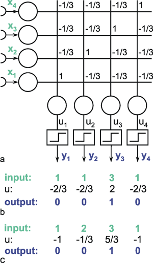
Fig. 10.6 A feedforward winner-take-all network (a). The weights at the diagonal are 1. Because the net consists of four neuroids in each layer, all other weights have a value of -1/3. (b) and (c) show two examples of input values (upper line), the corresponding summed excitations ui (middle line) and the output values after having passed the Heaviside activation function (lower line). In the example of (b) the threshold of the activation function could be any value between -2/3 and 2. For (c) this threshold value has to lie between 1/3 and 5/3
The winner-take-all network detects the maximally stimulated unit. This means that the unit with the highest input excitation obtains an output of 1 whereas all other units show a zero output.
The systems dealt with so far are characterized by the fact that the weights are prespecified and repeated for each neuroid in the same way. Below, the properties of those feedforward nets will be addressed in which the weights are distributed in an arbitrary way. This will be demonstrated using the simple example of a structure called "learning matrix" by Steinbuch (1961) , but without actually dealing with the learning itself at this stage. A simple example is shown in Figure 10.7. The net contains six neuroids at the input and four neuroids at the output. Subsequently, these output signals are fed into a winner-take-all net which has the function discussed above of merely detection the maximally stimulated channel. The weights can only take values +1 or -1, and have been arranged in the manner shown in Figure 10.7a. The figure shows four different input patterns on the left. These could be interpreted, for example, simply as an excitation of a linearly arranged group of photoreceptors or mechanoreceptors, or as the excitation of six different sense organs. When these four patterns are introduced into the net one after the other, the result is that, for each of the patterns, one of the four output channels is maximally stimulated, i. e., to value 6. The table in Figure 10.7b shows the corresponding values. According to the winner-take-all net, one specific neuroid will thus respond by showing value 1, the others by showing zero. One could thus state that this network distinguishes between these four input patterns and responds to each with a different reaction.
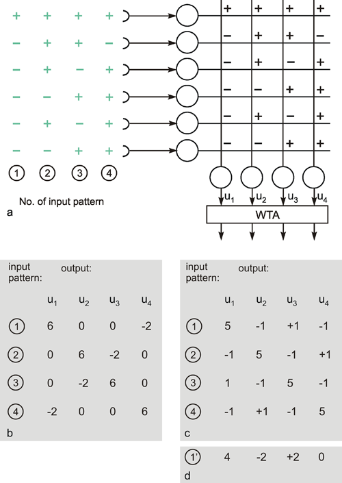
Fig. 10.7 The "learning matrix," a two-layer feedforward net. Input values and weights consist of either 1 or -1, but only the signs are shown. Four different input patterns are considered, numbered from 1 to 4 (left). (b) The summed values u; obtained for each input pattern. After passing the winner-take-all net, (Fig. 10.6, threshold between 0 and 6), only the unit with the highest excitation shows an output value different from zero. For each pattern, this is a different unit. (c) As (b), but the lowest input unit is assumed not to work. The winner-take-all net shows the same output as in (b), if the thresholds of the winner-take-all net units lie between 1 and 5. (d) The u; values obtained when a pattern 1' similar to pattern 1 (the sign of the lowest unit is changed) is used as input pattern. The output is the same as for pattern 1, if the thresholds lie between 2 and 4
The interesting property is that the net retains this ability even if, for some reason, one of the neuroids at the input ceases functioning. For instance, should the lowest input channel in Figure 10.7a fail, pattern 1 would, at the four outputs, exhibit the following values: 5, -1, 1, -1 and thus still be able to detect the right answer (Fig. 10.7 c). This property is sometimes referred to as graceful degradation. Moreover, the system responds tolerantly to inaccuracies in the input patterns. For example, if pattern 1 is changed in such a way that the sixth position shows +1 instead of -1, the outputs exhibit the following values: 4, - 2, 2, 0, and these still give the proper answer (Fig. 10.7d). Thus, the system does not only tolerate internal, but also external errors, i. e., "errors" in the input pattern. The latter may be also described as a capacity for "generalization," since different patterns, provided they are not too different, are treated in the same way. For this reason, such systems are also called classifiers. They attribute a number of input patterns to the same class. The properties of error tolerance and generalization become even more obvious when the system is endowed with not just a few (as in our example for reasons of illustration) but many parallel channels. While the example chosen here, showing six input channels, will break down if three channels are destroyed, such an event will naturally have much less effect on a net with, say, a hundred parallel channels.
This system can also be regarded as information storage or memory. In a learning process, information on specific patterns, four in our example, has been stored in the form of a particular distribution of weights. This learning process will be described in Chapter 12 in detail, but it will not have escaped the reader that the weights correspond exactly to the patterns involved. These patterns are "recognized" after being put into the net. Here, the storage or input of data is not, as in a classical computer, realized via a storage address, which then requires the checking of all addresses in turn to locate the required data. Rather, it is the content of the pattern itself which constitutes the address. This type of memory is therefore known as content addressable storage. In addition to the properties already mentioned of error tolerance, this kind of storage has the advantage that, due to the parallel structure, access is much faster than in classical (serial) storage.
A distributed network can store information by appropriate choice of the weight values. In contrast to the traditional von Neumann computer, it is called a content addressable storage. The system can be considered to classify different input vectors and in this way shows the property of error tolerance with respect to exterior errors ("generalisation") and interior errors ("graceful degradation").
A network very similar to the learning matrix is the so-called perceptron ( Rosenblatt 1958 ), which was developed independently at about the same time. The main difference is that in perceptron not only weights of the two values -1 and +1 are admissible, but also arbitrary real figures. This necessarily applies to the output values as well, which subsequently, however, at least in the classical form of the perceptron, are transformed by the Heaviside characteristic, thus eventually taking value 0 or 1. The threshold value of the Heaviside function is arbitrary but fixed.
The properties of such a network can be easily understood when some simple form of vector calculation is used. The values of the input signals x1 ... xn can be conceived of as components of an input vector x, and similarly the weight values of the j-th neuron of the output layer w1j ... wnj, can be conceived of as components of a weight vector w j. The output value of the i-th neuron before entering the Heaviside function is calculated according to ui =jΣ wij xj. ui would then be the inner product (= scalar product, dot product) of the two vectors. The value of the scalar product is higher, the more similar the two vectors are. (It corresponds to the cosine of the angle between both vectors if both vectors have the same unit length.) The highest possible value is thus reached when both vectors agree in their directions. ui can thus also be understood as a measure of the strength of the correlation between the components of both vectors. Such a feedforward net would thus "select," i. e., maximally stimulate, that neuroid of the output layer whose weight vector is the most similar to the vector used as input pattern. The numerical examples given in the table of Figure 10.7 illustrate this. The function of the Heaviside characteristic is to ensure that only 0 or 1 values appear at the output. However, as mentioned earlier, the appropriate amount of the threshold value is critically dependent on the range of the input values. A better solution is given by using a recurrent winner-take-all net as described later.
A simple perceptron with only one single neuroid in the output layer would constitute a classifier that assigns all input patterns to one of two classes. Minsky and Papert (1969) were able to show that the capacity of this system for assigning a set of given patterns to two classes is limited. For example, it is not possible to assign all those patterns in which the number of input units showing +1 is even to one class, and all other patterns in which the number of input units showing +1 is odd to the other class (the so-called parity problem). On the other hand, many of the problems associated with the perceptron can be solved, if the net is endowed with a further layer, i. e., has a minimum of three layers. This will be explained in more detail in Chapter 10.7 .
Looking at a net endowed with m inputs and n outputs, the inputs, as mentioned above, can be interpreted as representations of different sensory signals, and the outputs as motor signals. The systems thus associates stimulus combinations to specific behavior responses. Since the output pattern and the input pattern, which are associated here, are usually different, we speak of a heteroassociator.
The output of a unit of a two-layered feedforward network can be determined by the scalar product between the input vector and the weight vector of this unit. This product is greater the stronger the components of both vectors correlate. Different input vectors produce different output vectors. This is sometimes described as heteroassociation.
As already mentioned, multilayer nets, i. e., nets endowed with at least one "hidden" layer, exhibit some properties that are qualitatively new compared to two-layer nets. Two-layer nets can solve only problems which can be linearly separated. To show this we will use a simple example that is not linearly separable, namely the XOR problem. Solving this task requires a system with two input channels and one output channel, which should behave in the way shown in the table of Figure 10.8a2. The problem will be explained by representing the four input stimuli, i. e., the four two-dimensional vectors, in geometric form. According to the XOR task, these four vectors, which are shown in Figure 10.8a3 geometrically in terms of their end points, are to be divided into two groups. This cannot be done linearly, i. e., by a line in this plane, since the two points which belong to the same class are located diagonally from each other. Other problems, e. g., the AND problem, are linearly separable and, for this reason, can be solved by way of a two-layer net, here consisting of a total of three neuroids (see Figure 10.8b). In this example, both weights are 1 and the threshold of the Heaviside characteristic is 1.5. The XOR problem can be solved only if a hidden layer is introduced, which, in this simple case, need only contain a single neuroid (Fig. 10.8c). The neuroid of the hidden layer is connected in such a way with the input units that it solves the AND problem. The output neuroid is then given three inputs which are shown in the table of Figure 10.8c2. The vector influencing the output neuroid is now three-dimensional, necessitating a spatial representation of the situation. As shown in Figure 10.8c3, the problem is now a linear one, i. e., separable by an oblique plane, and can be solved. By using the weights and threshold values shown in the network of Figure 10.8c1, the required associations can be obtained.
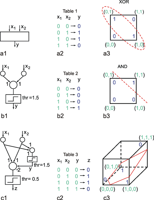
Fig. 10.8 The XOR problem. (a1 ) A system with two input units and one output unit should solve the four tasks presented in the Table (a2). These tasks are illustrated in geometrical form (a3) such that the four input vectors are plotted in a plane and the required output values are attached to their input vectors. The two input vectors which should produce an output value of one are circled. (b1 ) A two-layer system solving the AND problem. As in (a), the tasks to be solved are shown in Table (b2) and in geometric form in (b3). The network (b1) can solve the AND problem using the weights shown and a Heaviside activation function with a threshold of 1.5. (c) A three-layer system can solve the XOR problem, when, for example, the weights and threshold values shown in (c1) are applied. The output y of the hidden unit corresponds to that of the AND network (b1) (see Table c2). The input vector of the final neuroid, representing the third layer, is three-dimensional. Therefore, geometrically the input-output situation of this unit has to be illustrated using a three-dimensional representation. As above, the four input vectors are marked together with the expected output. The oblique plane separates the two vectors producing a zero output from the two others which produce unity output. Such a linear separation is not possible in (a3)
Thus, in some cases, hidden neuroids have to be introduced for logical reasons. It is also conceivable, though, that hidden neuroids are not required for the solution of a given problem, but that a net may become less complex, need fewer channels, and that individual neuroids could be interpreted as to have a symbolic significance. Figure 10.9 provides a good, although somewhat artificial, example, namely a simulation of Grimm's Little Red Riding Hood ( Jones and Hoskins 1987 ). In Figure 10.9a Riding Hood is simulated using a two-layer net. As we know, Riding Hood has to solve the problem of how to recognize the wolf, the grandmother, and the woodcutter and respond appropriately. To this end, she possesses six detectors which register the presence or absence (values of 0 or 1) of the following signals of a presented object: big ears, big eyes, big teeth, kindliness, wrinkles, handsomeness. If Riding Hood detects an object that is kindly, wrinkled, and has big eyes, which are supposed to be the features of grandmother, she responds by behaving in the following ways: approaching, kissing her cheeks, offering her food. With an object that has big ears, big eyes, and big teeth, and is probably the wolf, Riding Hood is supposed to run away, scream, and look for the woodcutter. Finally, if the object is kindly, handsome, and has big ears, like the woodcutter, Riding Hood is supposed to approach, offer food, and flirt. The net shown in Figure 10.9a can do all this, if the existence or nonexistence of an input signal is symbolized by 1 or 0 and, correspondingly, the execution of an activity by 1 instead of 0 at the output.
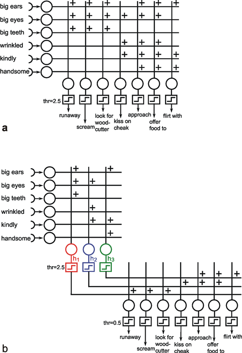
Fig. 10.9 Two networks simulating the behavior of Little Red Riding Hood. Input and output values are either zero or one. (a) In the two-layer net the thresholds of the Heaviside activation functions are 2.5. (b) For the three-layer network threshold values are 2.5 for the hidden units h1, h2, and h3 and 0.5 for the output units
Instead of a two-layer net, a three-layer net can also be used to simulate Riding Hood. This is shown in Figure 10.9b, with a middle (hidden) layer consisting of three neuroids. The question of how the values of the weights of both nets are obtained, i. e. the question of learning, will be discussed later. Both nets, the two-layered and the three-layered net, obey the same input-output properties but there are differences when the internal properties are considered. First, the three layered net requires fewer cross-sectional channels, i. e., number of weights per layer (a maximum of 21 in Figure 10.9b, compared to 42 in Figure 10.9a). Secondly, and this is especially interesting, a symbolic meaning can be attributed to the three hidden neuroids. Neuroid h1 obtains a high excitation, if the features of the wolf are displayed at the input. The same applies to neuroid h2 in relation to Grandmother, and to neuroid h3 regarding the woodcutter. It is thus possible that intermediate neuroids can collect different, but qualitatively interrelated data, and can in this way be interpreted as symbols or concepts for the object concerned. If, as described later, these connections are learnt, one could argue that the system has developed an abstract concept of exterior world. It should, however, be mentioned here that the idea of the "grandmother cell" is intensively disputed in neurophysiology.
If, as an activation function, one includes not only the Heaviside function, but also linear or sigmoid ("semilinear") functions, both input and output values may take arbitrary real values. Generally, such a system exhibits the following property. It maps points from an n-dimensional (input) space onto points in an m-dimensional (output) space, thus representing a function. This could be a continuous function, whereas networks with Heaviside characteristics (see earlier examples in this chapter and also some recurrent networks) form functions with discrete output values. It can be shown that a net with at least one hidden layer can represent any function, provided it is integrable. A given mapping becomes more precise the greater the number of neuroids in the hidden layer. However, increasing the number of the hidden units can also provide problems as discussed in Chapter 12 .
In the following, an example of such a mapping will be presented in which a two-dimensional subset of a three-dimensional space is mapped onto a two-dimensional subset of another three-dimensional space. During walking, some insects can be observed placing three legs of one side of their body in nearly the same spot. It can be shown that the reason for this is that the spatial position of the foot of one leg is signaled to the nearest posterior leg, which then makes a movement directed to this point. The foot's position is determined by three joints and hence three variables α, β, and γ. The system, which transmits the information from one leg to the next, thus, requires at least three neuroids in the input layer (Fig. 10.10a) ( Dean 1990 ). These may correspond to the sense organs which measure the angles of the joints of the anterior leg. Furthermore, three neuroids are required in the output layer, serving to guide the three joints of the posterior leg. Since, in this model, only foot positions are considered which lie in a horizontal plane, only two dimensional subsets of the three-dimensional spaces, which are generated by a leg's three joint angles, need to be studied. Figure 10.10b shows the behavior of the system in which three neuroids are given in the hidden layer. Circles show the given targets, crosses the responses of the net. The length of the connecting lines are thus a measure of the magnitude of the errors, which still occur when using only three hidden units.
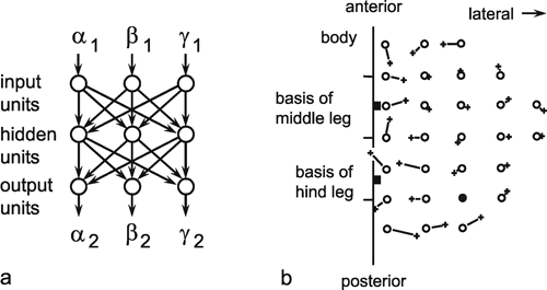
Fig. 10.10 (a) A three-layer net which determines the position of an insect hind leg with three joints (given by the joint angles (α2, β2, γ2), when the joint angles of the insect's middle leg (α1, β1, γ1) are given. The logistic activation functions are not shown. (b) Top view of the positions of the middle leg's foot (circles) and that of the hind leg (crosses). Corresponding values are connected by a line showing the size of the errors the network made for the different positions (after Dean 1990 )
This example illustrates the case of a continuous function. But it could be shown that such a net can also approximate mappings which, rather than having to be continuous, have only to be integrable, i. e., exhibit discontinuities.
Three (or more) layered feedforward networks can solve problems which are not linearly separable. Hidden units might represent complex (input) parameter combinations. A multilayered feedforward network constitutes a mapping from an m-dimensional sensor space to an n-dimensional action space (m, n: number of input and output units, respectively).
As mentioned above, nets with feedback connections constitute the most general version because, by setting specifically chosen weights to zero, they can be transformed into any form of feedforward net. if feedback connections are present, the nets may have properties which do not exist in a simple feedforward net. This will be demonstrated using a fairly simple example, namely a net consisting of two neuroids. Saturation characteristics are assumed as activation functions (Fig. 11.1 a). These have the effect that the output values are restricted to the interval between +1 and -1. What output values can be taken by this system? All conceivable states (y1, y2) can be represented in a two-dimensional state diagram (Fig. 11.1 b) by plotting the output values of the two neuroids along the coordinates. Any point in the plane corresponds to a potential state of the system. The system is characterized by the fact that only two states, namely state (+1, -1) and state (-1, +1), are stable. All other states are unstable. This means that by an appropriate selection of the input values a specific state of the system can be brought about, but that, in the course of time, the system will by itself pass into one of the two stable states. The easiest way to understand this is to calculate this behavior by using concrete numerical examples. The state of the neuroids at time t + 1 can be determined according to the equations


with w21 = w12 = -1 and w11 = w22 = 1. The input signal is turned off (set at zero) after the first cycle.
If one starts with state (+ 1, -1), this state is maintained for each subsequent cycle. If one starts, for example, with (0.5, 1), the resulting states are (-0.5, 0.5) (-1,1) (-1,1)... This means that the stable state is reached by the second time step. For other starting points the "relaxation" to a stable solution might take longer. Starting with (-0.2, 0.2), for example, yields (-0.4, 0.4), (-0.8, 0.8), (-1,1) as illustrated in Figure 11.1 b. All states y1 = y2 (e. g., 0.4, 0.4 or 0,0, see dashed line in Figure 11.1 b) belong to a special case. They represent an unstable equilibrium which ceases whenever there is a slight disturbance.
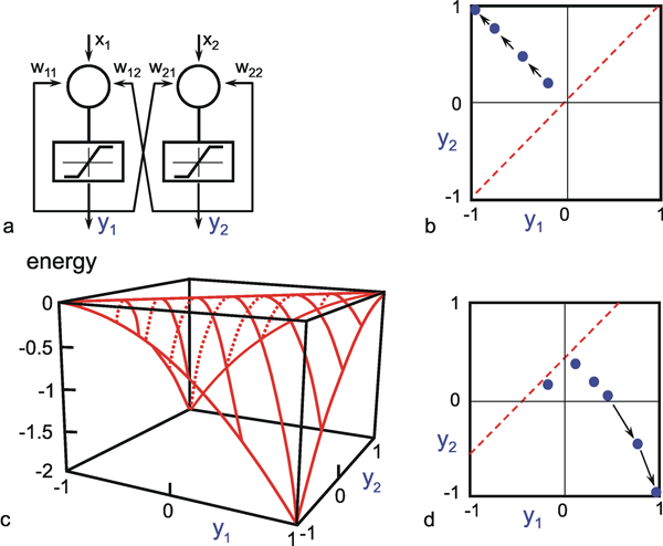
Fig. 11.1 (a) A recurrent network consisting of two neuroids. (b) The temporal behavior of the system shown in the state plane determined by the output values y1 and y2 , starting with (-0.2/0.2). The dashed line separates the two attractor domains. (c) The energy function of the system. The energy (ordinate) is plotted over the state plane. (d) as (b) but using offset values θ1 = 0.5 and θ2 = 0. The (dashed) borderline between the two attractor domains is shifted and the system now finds another stable solution for the same input
The behavior of this system can be illustrated using an energy function introduced by Hopfield (1982) . The "energy" of the total system is calculated as follows:
 ,
,
or, if the neuroids contain an offset value θi,

(This offset value is sometimes misleadingly called threshold). In our case of two neuroids, this leads to E = -1/2 (w12y1y2 + w21y2y1 + w11y1y1 + w22y2y2).
For w12 = w21 = -1 and w11 = w22 = 1 we obtain E = - ½ (y1 – y2)2 . The area defined by this function is shown in Figure 11.1c. The system's behavior is characterized by the fact that it moves downward from any initial state and, in this way, reaches a state of rest at one of the two lowest points, i. e., (+1, -1) or (-1, +1). These states are therefore known as states with the lowest energy content, or as attractors. Such an attractor can be interpreted as representing a pattern stored in the net. Each attractor has a particular domain of attraction. Accordingly, the system becomes stabilized at that attractor in whose domain the initial state of the system was observed.
Near the borderline between two attractor domains (dashed line in Figure 11.1b) the classical rule "similar inputs produce similar outputs" no longer holds. Small changes of the input signal may produce qualitative changes in the output. States where such “decisions” are possible are eventually termed bifurcation points. Such a network may also be regarded as a kind of distributed feedback ontrol system because it shows an inherent drive trying to push the system in its attractor state. In this case the reference signal is not explicitly given but corresponds to the attractor of the domain of the actual input vector. The disturbance corresponds to the deviation of the input vector from the attractor. It should be noted at this point that, depending on the problem involved, other energy functions can also be defined (see Chapter 11.3 for an example). Other names for these energy functions are Lyapunov functions, Hamilton functions, cost functions or objective function.
The form of this energy plane can be altered by selecting different weight values, or by the fact that input values are not switched off, but remain permanently switched on. This corresponds to an alteration of the offset values of the neuroids. In this way, the size of the domain of attraction can be changed, and with it, of course, the behavior of the system. If, for example, θ1 = 0.5 and θ2 = 0, the range of the attractor 1, -1 becomes larger, and its minimum lower than those of the attractor -1, 1 (Fig. 11.1d). The borderline is shifted as indicated in Figure 11.1d. Starting at (-0.2, 0.2), the state will now change to (0.1, 0.4), (0.2, 0.3), (0.4, 0.1), (0.8, -0.3), and (1, -1), and therefore reach the other attractor.
The concept of an energy function can also be used if the system is endowed with more than two neuroids. This is generally known as a Hopfield net. In such a net, the activation function of neuroids may be linear in the middle range, or nonlinear, but has to show an upper and a lower limit. A further condition, and thus a considerable limitation of the structure of Hopfield nets, is that connections within the net must be symmetrical, i. e., wij = wji. This precondition is required so that the energy function introduced by Hopfield can be defined. Detailed rules describing the behavior of nonsymmetrically connected nets in general are as yet unknown.
On account of the symmetry condition, the number of potential weight vectors, and thus the number of potential patterns, is lower than the maximum number of patterns that could be represented by a net of n neuroids. The symmetry condition follows from the application of Hebb's Rule in storing the patterns (see Chapter 12.1 ). Moreover, with this assumption, it is easy to define the energy function in question. Assuming that the patterns show a random distribution, i. e., that about half of the neuroids take value 1 and the other half value -1, one can store maximally n/(4 log n) patterns in a net consisting of n neuroids, if, after recalling the pattern, this pattern is to be generated without errors. If an error of 5% is tolerated, the maximum figure is 0.138 n. The reason for assuming randomness of distribution is that, in this case, no correlation is observed between the patterns. If correlation exists, cross talk is greater and the capacity of the net smaller, accordingly. (A special case of nonrandomness of distribution is present, if the patterns are orthogonal in relation to each other (see Chapter 12 . At most n patterns can then be stored and recalled without error.)
If a net is endowed with n recurrently connected neurons, the energy function is defined within an n-dimensional space. It may then exhibit a higher number of minima, i. e., attractors and their domains of attraction. The depth of the minima and their domains of attraction may greatly vary. Undesirable local minima may also occur, known as spurious states. Usually, Hopfield nets are considered in which wii = 0, i.e. there are no connections of a neuroid onto itself. This is, however, not necessary. Positive values of wii reduce the number of spurious states by slowing down changes of the activation values of the neuroids because thereby the dynamic of a temporal low-pass filter is introduced (see Chapter 11.5 ).
An important property usually applied in the Hopfield nets is that updating of the neuroids is not performed in a synchronous manner. Although synchronous updating was used in the above example (Fig. 11.1), asynchronous updating corresponds more to the situation of biological systems. A synchronous system is easier to implement on a digital computer but requires global information, whereas in biological systems only local information is available. Asynchronous updating can be obtained, for example, by randomly selecting the neuroid to be updated. However, the following examples will use synchronous updating which can be considered as a special case of asynchronous updating.
Recurrent networks constitute the general form of networks. However, only special versions can be understood at present. For symmetrical networks (wij = wji) an energy function can be formulated which illustrates the behavior of such a net. For any input vector, the net "relaxes" to one of several stable states ("attractors") during a series of iteration cycles. This attractor corresponds to a minimum of the energy function.
First, a recurrent net will be studied in which the weights of each neuroid are arranged in the same manner. This means that, apart from the neuroids at the margin of the net, each neuroid is connected to its neighbors in the same way. The net's structure is thus repetitive. With adequate connections, the network is then capable of forming stable excitation patterns.
In biological systems, pattern generation is a frequently encountered phenomenon, e.g., the formation of stripe patterns in skin coloring, or the arrangement of leaves along the stem of a plant. Another problem concerning an organism's ontogenesis is posed by the generation of polarity without external determining influences being present. When the body cells of Hydra are experimentally disconnected and mixed up, an intact animal will be reorganized from this cell pile such that after some time one end of the heap contains only those cells that form the head of the animal and the other contains those that form its foot. How can the chaotic pile of cells of a Hydra become an ordered state? Assuming that the individual cells spontaneously choose one of the two alternatives, namely +1 and -1(i. e., "head" or "foot" cell), the formation of the desired polarity is possible as follows. Each "head cell" emits a signal, stimulating growth of the head, to the neighboring cells and another signal, inhibiting growth of the head, to the more distant cells. The corresponding applies to each "foot cell". These mechanisms can be simply demonstrated using a recurrent network. (Of course, the connections are not formed by axons and dendrites in this case. Rather, the cells send hormone-like substances and, by means of diffusion and possibly decomposition, the concentration decreases with distance from the sender.) One assumes that each cell is represented as a neuroid which is linked to its direct neighbors via positive weights, corresponding to excitatory substances, and to its more distant neighbors via negative weights, which correspond to inhibitory substances. The neuroids summate all influences and then "decide," with the aid of a Heaviside activation function, whether they are going to take value +1(for head) or -1 (for foot) at the output. Figure 11.2 shows the behavior of the system, after an appropriate choice of distributions of inhibitory and excitatory weights. After only a few time steps, a stable pattern develops from the initially random distribution of head and foot cells such that, at one end only head cells are to be found, whereas the other end shows only foot cells. Depending on the initial state, the final arrangement may also be exactly reversed. Thus the system has two attractors. If the weight distribution is chosen in such a way that coupling width is less than that for the system shown in Figure 11.2, periodic patterns may also result. One could say, therefore, that these systems are characterized by the fact that, by self-organization (i. e., on the basis of local rules) they are capable of generating a global pattern. It should be mentioned that such neuroids with Heaviside characteristics and connected by local rules can correspond to systems often described as cellular automata.

Fig. 11.2 Development of an ordered state. The recurrent net consists of 20 units which can take values of 1 or -1. Only the signs are shown. The first line shows an arbitrary starting state. During the four subsequent time steps (iteration cycles t2 - t5) the net finds a stable state. Positive output values are clustered at the left and negative values at the right. For another starting situation the final state may show the cluster of positive values on the right side
With appropriately chosen weights, a recurrent network can show the formation of spatial patterns. This can be considered as an example of self-organization.
Diffusion Algorithms
Diffusion is an important phenomenon because it forms the basis of many physical processes. Furthermore, the diffusion analogy can also be used to understand other processes as explained below. To describe those processes, the so-called reaction-diffusion differential equations often are used. However, diffusion can also be simulated using artificial neural nets.
As an example we will first consider the simulation of diffusion in a two-dimensional space. For this purpose, we represent this space by a two-dimensional grid of neuroids that obey recurrent connections with direct neighbors. This is shown in Figure B5.1a, b. In (a), the top view is shown, and in (b), a cross section illustrating the connections between the neuroids i -1, i, and i + 1 is shown. The neuroids are arranged in the form of a hexagonal grid. Therefore, each neuroid has six neighbors. All weights are w = 1/6 except for those neuroids that coincide with the position of an obstacle (see below). To start the simulation, one neuroid is chosen to represent the source of a, say, gaseous substance. This neuroid receives a constant unit input every iteration cycle. As a result, a spreading of excitation along the grid can be observed (Fig. B5.1 c). This excitation, in the diffusion analogy, corresponds to the concentration of the diffusing substance, forming a gradient with exponential decay along the grid. (The exponential decay could be linearized, if this is preferred, by introduction of a logarithmic characteristic f(u) to compensate the exponential decay. In our example, however, f(u) is linear). Figure B5.1 c shows the result of such a diffusion which was, in this case, produced in a nonhomogeneous space: Some parts of the grid are considered as tight walls, which hinder the diffusion of the substance, i,e., connections across these walls are set to zero. The position of these walls is shown by bold lines. After 5000 iteration cycles, the excitations of the neuroids form a surface as shown.

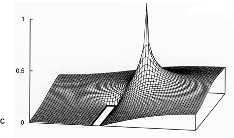
Fig. B 5.1 Top view of a small section of the two-dimensional hexagonal grid. Each unit is connected with its six direct neighboring units. (b) Cross section showing those three units and their recurrent connections which, in (a), are marked by bold lines. The weights are w = 1/6. (c) The excitation of the units after 5000 iteration cycles. The bold rectangle marks an obstacle ( Kindermann et al. 1996 )
Such a gradient could be applied, for example, to solve the problem of path planning in a plane cluttered with obstacles. In this case, the goal of the path is represented by the diffusion source. The walls represent the obstacles. The path can start at any other point in the grid. The path-searching algorithm simply has to step up the steepest gradient in this "frozen" diffusion landscape. If paths exist, this procedure finds a path to the goal, for any arrangement of the obstacles ( Kindermann et al. 1996 ).
As another example, the development of an epidemic disease, such as rabies, can be considered. Figure B5.2 shows the spotty spatial distribution of rabies carried by foxes in Europe. This development is assumed to have begun in Poland in about 1939. Rabies also shows a temporal cyclic pattern with a new epidemic appearing every 3-5 years at a given local position. This can be understood by representing the area using a two-dimensional grid, the excitation of the neuroids representing the intensity of infection of the corresponding local area. First of all, there is a diffusion process of spreading the infection as described above. However, a further mechanism is necessary. After infection in an area has reached a given threshold, self-infection leads to an almost complete infection of that area. This can be simulated by a recurrent excitation of the corresponding neuroid and an activation function with a saturation, describing the fully infected state. With these mechanisms, the infection would spread out over the grid like a wave front. There is, however, a third, important phenomenon. When an area is heavily infected, the foxes die from the disease and therefore the number of infected foxes in this area decreases to about zero. This "reaction" can be simulated by each neuroid being equipped with high-pass properties, or by application of an additional neuroid as shown in Figure 11.8. When the time constant of this high-pass is chosen appropriately, spatial and temporal rhythmical distributions can be found in this simulation of a reaction-diffusion system, which very much correspond to those found in nature. Exceptional cases of further examples can be found in Meinhardt (1995) .
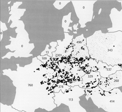
Fig. B 5.2 Spotty distribution of rabies (dots) in central Europe in the year 1983. In brackets: number of counts. The data from Poland and the former DDR are not comparable with the others because they were collected over larger spatial units (after Fenner et al. 1993 ; courtesy of the Center for Surveillance of Rabies, Tübingen, Germany)
In the following example, other local rules have been applied. The cells are arranged in an orthogonal grid and each cell is connected with its eight neighbors. Each cell can adopt three different states of excitation (shown by white, gray, and black shading). The system is started with a random distribution of these states. The local rules are as follows: if a cell is in state 1 and three or more neighboring cells are in state 2, the cell adopts state 2 in the next iteration cycle. Correspondingly, if a cell is in state 2 (3) and three or more neighbors are in state 3 (1), the cell adopts state 3(1). After some time, a picture results similar to that shown in Figure B5.3. These spirals are not static, but change their shape with time, increase their diameters, seem to rotate, and merge with other spirals. The temporal behavior of this structure reminds one of the rotating spirals that can be observed during the growth of some fungi species. For the sake of simplicity, the local rules used here a formulated by logical expressions, but could be reformulated for an neuronal architecture.
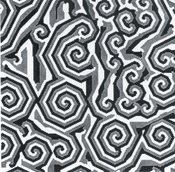
Fig. B 5.3 A snapshot of moving spirals (Courtesy of A. Dress and P. Sirocka)
As mentioned above ( Chapter 10.4 ) a winner-take-all network can also be constructed on the basis of a recurrent network. As shown in Figure 11.3a, this can be obtained when each neuroid influences itself by the weight 1 and all other neuroids by the weight -a. In general, if the system is linear, the output values of this net will oscillate. If, however, half wave rectifiers are used as activation functions, the system shows better properties than the feedforward winner-take-all net. Even for small differences between the input values, the net always produces a unique maximum detection. The higher the value of a, the faster the winner appears, which means that all output values except for one are zero. If the value of a becomes too great, oscillations might occur. The optimal value is a = 1/(n-1) for a net consisting of n neuroids. Figure 11.3b shows a formally identical net in which a special neuroid is introduced to sum all output values. This value is then fed back, which requires a smaller number of connections.
Compared to the feedforward system, the recurrent winner-take-all net shows the same properties but behaves as if it could adjust its threshold values appropriately for the actual input values. The behavior of the recurrent system can be made clear by imaging instead a chain of consecutive feedforward winner-take-all nets. Each such feedforward net corresponds to a new iteration cycle of the recurrent system. Using this so-called "unfolding of time," any recurrent network can be changed into an equivalent feedforward network.
A recurrent winner-take-all net can be used in two ways. First, the input vector can be clamped continuously to the system during the relaxation. Alternatively, the input vector can only be given into the system for the first iteration cycle and then switched off. In the second case, relaxation is faster and the value of the winner becomes stable. However, the value of the winner is small when the difference between the input values is small. In the first case, the value of the winner increases steadily with the iteration cycle. In both cases the problems can be solved when an additional neuroid is introduced to normalize the sum of all output values to 1. The output of the extra summation unit shown in Figure 11.3b can be used for this purpose. An example of a recurrent winner-take-all net with nonhomogeneous connections is given in Figure 15.2.
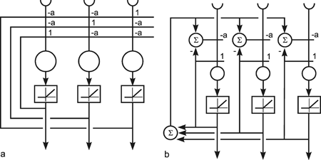
Fig. 11.3 A recurrent winner-take-all network consisting of three units (a). A formally identical system with four extra units (b). Rectifiers (Fig. 5.8) are used as activation functions
Using a recurrent structure, winner-take-all nets can be constructed having more convenient properties than those based on a feedforward structure.
As we have seen, recurrent nets with a given weight distribution are endowed with the property of decreasing from an externally given initial state to a stable final state, i. e., "relaxing." This property could also be useful in solving optimization problems. This will be illustrated by the following example ( Tank and Hopfield 1987 ). Let us assume that we have six subjects to solve six tasks. Each subject's ability differs in relation to the various tasks. To illustrate this, each line in the table of Figure 11.4a shows the qualities of one subject in relation to the six tasks, in numerical terms. The question arises as to which subject should be assigned which task to ensure that all the tasks will be optimally solved. There are 6! (= 720) possible solutions. The problem can be presented in the form of a net as follows: For each subject and each skill a neuroids is used with a bounded activation function (e.g., tanh ax, see Fig. 5.11b). The best way to arrange these 36 neuroids is in one plane as shown in Figure 11.4a, i.e., to arrange those neuroids representing the skills of one person in a line, and those representing the same skills of the various subjects in a column. Since each task is undertaken by only one subject, the neuroids in each column have to inhibit each other (this forms a recurrent winner-take-all subnet). Correspondingly, since each person can only do one task, the neuroids in each line have to inhibit each other. So far, each neuroid is linked with some but not all of the other neuroids in the net. A third type of linkage, however, has to be introduced which requires global connections. As for the final solution, exactly six units should be excited, the sum of all units is computed, and the value 6 is subtracted from this sum. This difference, which for the final solution ought to be zero, is then fed back with negative sign to all 36 units. These last connections can be interpreted as forming for each unit, a negative feedback system, the reference input of which is zero.
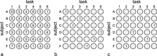
Fig. 11.4 Six subjects A - F have to perform six tasks 1-6. To solve the optimization problem, 6 x 6 units are arranged in six lines, one for each subject (a). The vertical columns correspond to the tasks to be performed. The number in each unit shows a measure for the qualification of each subject and each task. These numbers represent the input values. The units are connected such that the six units of a line as well as the six units of a column form winner-take-all nets. Furthermore, an additional unit computes the sum of the activations of all these 36 units (as shown in Fig. 11.3b) including an offset value. This sum is fed back to all 36 units. (b) An almost optimal solution found by this network. The sum of the qualification measures is 40 in this case. The optimal solution is shown in (c) with a total qualification of 44 ( Tank and Hopfield 1987 )
Each of the 720 possible solutions represents a minimum of the energy function of the net. This energy function is defined in a 36 dimensional space. (In the example of Figure 11.1 we had an energy function defined in a two-dimensional space with two minima.) Taking into account the known qualities of each subject, the problem consists of finding the combination that ensures the highest overall quality, i.e. the largest possible sum of selected qualities. To achieve this, the individual quality values are given as an input to the 36 neuroids. This influences the energy plane of the net in such a way that the lower the minimum of individual solutions, the better is the corresponding solution. The net then selects, either the best or one of the best solutions. Figure 11.4b shows an almost optimal, and Fig. 11.4c by comparison, the best, solution to this problem.
However, it should be mentioned that the Hopfield net is not generally appropriate for the solution of optimization problems when the number of neuroids increases, because the number of local minima increases exponentially. There are methods which ensure that the net is not so easily caught in a local minimum. In principle, this is achieved by introducing noise on the excitation of the individual neuroids. In this way, the system is also capable of moving to a higher energy level and thus of eventually escaping from a local minimum. Noise can be introduced by simply adding a noisy signal on the neuroid before the activation function is applied. An alternative method is to use probabilistic output units. These can take either 0 or 1 as output value, and the input value determines the probability, whether the output will be 0 or 1. This probability is usually described by the logistic function (Fig. 5.11b). Such a probabilistic system is called a Boltzmann machine. This will not be discussed here (for more details see e. g., Rumelhart and McClelland 1986 ). Yet another possibility to introduce noise is to use asynchronous updating with randomly selecting the unit to be updated.
At least for networks with a sufficiently small number of units and appropriately chosen cost function (represented by the proper weight distribution), recurrent nets can be used to search for optimal solutions.
Apart from pattern generation and optimization, the most frequently discussed application of recurrent nets is their use in information storage. According to the distribution of weights several patterns can be stored. As with feedforward nets, autoassociation, (i, e., where the input pattern also occurs at the output) as well as heteroassociation can be performed with recurrent nets. In the latter case, a pattern occurs at the output which differs from that at the input. The net can also be used as classifier, which can be regarded as a special case of heteroassociation. We use the term classification, if only one of the neuroids of the output pattern takes value 1 and the remaining (n - 1) ones take value zero.
Generally, the storage constructed on the basis of recurrent nets is endowed with the same properties described earlier for feedforward nets. They are error-tolerant, since a stable output pattern corresponds to an energy minimum. For this reason, the attractor is also reached, if the input pattern does not correspond exactly to the correct pattern. The domain of an attractor could thus also be defined as a domain of tolerance or of generalization. Error tolerance also includes internal errors, e.g. the failure of individual weights or of a whole neuroid. This storage is also, of course, content addressable. Figure 11.5 provides an impressive representation of the properties of these nets. 20 patterns were stored in this Hopfield net, which consists of 400 neuroids with Heaviside activation functions. Figure 11.5b shows that after three time steps, one of these patterns is fully completed, even though only a relatively small part of this pattern was given as input. The same applies, when a noisy version of the original pattern is used as input pattern (Fig. 11.5c). Again, these examples demonstrate that, compared to a feedforward net, a recurrent net needs to perform a number of iterative steps, and thus a certain amount of time will elapse before it reaches its attractor. However, this apparent disadvantage can also be considered an advantage, as will be shown in the next section.
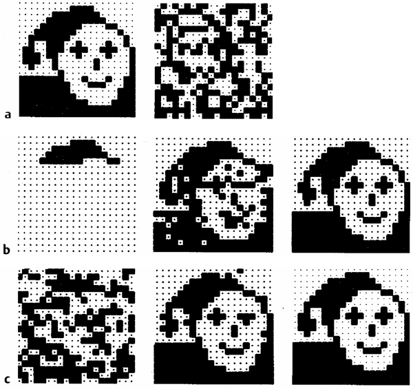
Fig. 11.5 Pattern completion. (a) The Hopfield net consists of 20 x 20 neuroids, which can show two states, illustrated by a dot or a black square, respectively. The weights are chosen to store 20 different patterns; one is represented by the face, the other 19 by different random dot patterns. (b) After providing only a part of the face pattern as input (left), in the next iteration cycle the essential elements of the final pattern can already be recognized (center), and the pattern is completed two cycles later (right). (c) In this example, the complete pattern was used as input, but was disturbed by noise beforehand (left). Again, after one iteration cycle the errors are nearly corrected (center), and the pattern is complete after the second iteration (right) ( Ritter et al. 1992 )
Like feedforward networks, recurrent nets can be considered as content addressable storage, which has the properties of error tolerance (generalization, graceful degradation).
A crucial disadvantage of feedforward nets has to do with their purely static character. A particular output pattern, which does not change over time, belongs to a particular input pattern. Recurrent nets, too, have so far usually been considered in this way. As a rule, however, biological systems are endowed with dynamic properties. The system responds to a particular input stimulus pattern with activities that change over time. As shown above, recurrent nets are in principle endowed with such properties. A particular input pattern is immediately followed by an output pattern, which changes over time until a final, stable state is reached. This property, which at first seems to be an undesirable one, can be utilized to produce time functions at the output. In this sense, the recurrent network shown in Figure 11.6 generates a rhythmic output when started by an input vector of (1,0,0), for example. The output vector then regularly cycles from (1,0,0) to (0,1,0), (0,0,1), (1,0,0) ...
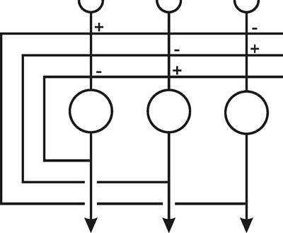
Fig. 11.6 An asymmetrical recurrent network showing rhythmic behavior. After the excitation of one unit, the three units are excited in cyclic order
Another simple system is shown in Figure 11.7a. This network is endowed with the property of a temporal low-pass filter. This becomes clear when the circuit, as shown in Figure 11.7b is redrawn. Due to its direct positive feedback, the second neuroid is endowed with the property of an integrator. The entire system (Fig. 11.7c) thus formally corresponds to an I-controller which, as shown in Figure 8.8e(Part I), can be regarded as a low-pass filter. If the integrator is placed in the feedback loop, the result is a temporal high-pass filter (Fig. 11.8, see also Part I - Figure 8.8f and Appendix II ). The circuit corresponds to that of Figure 11.7, although the output used here is that of neuroid 1 instead. In both cases the time constant is determined by the value of weight k (τ = 1/k).
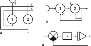
Fig. 11.7 An asymmetrical recurrent network with the properties of a temporal low-pass filter (a). (b) and (c) show the same system but are redrawn to allow comparison with figures of Chapter 8 (Part I) . For easier identification the two units are numbered in (a) and (b)
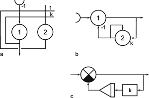
Fig. 11.8 An asymmetrical recurrent network with the properties of a temporal high-pass filter (a). (b) and (c) show the same system but are redrawn to allow comparison with figures of Chapter 8 (Part I) . For easier identification the two units are numbered in (a) and (b)
The nets shown in Figures 11.6 to 11.8 are endowed with an asymmetrical distribution of weights. Consequently, they no longer fulfill the conditions of a Hopfield net. In the following example, a further simple net with an asymmetrical distribution of weights will be used. Rhythmic movements, such as the movement of the wing of an insect in flight, or a fin during swimming, or a leg during walking, for example, are frequently not determined by an internal oscillator, as described in Figure 11.6. Rather, the reversal of the direction of a movement is often determined by a signal emitted by the sense organs in such a way that the registration of either of the two extreme positions triggers a reversal of the movement's direction. This behavior is simulated by the recurrent net shown in Figure 11.9. The output of the first neuroid represents movement in one direction, i. e., in the case of a wing it would activate the levator muscles, which raise the wings (US, upstroke). The second neuroid would, in turn, activate the depressor muscles, which lower the wings (DS, downstroke). The activity of these muscles thus results in a change of wing position. In a simplified way, this can be simulated by giving the outputs of both neuroids to an integrator with opposite signs. The wing position determined in this way is measured by two sense organs, but an excitation is transmitted only if either the lower extreme position (LEP) is reached (Heaviside characteristic at the input of neuroid 1), or the upper extreme position (UEP) is exceeded (similarly at neuroid 4). The integrator thus represents a simulation of the mechanical part of the total system. On the basis of the given weights, the net is endowed with the following properties. If all inputs are zero, activity ceases. If an excitation, i. e., an input of 1, is given to neuroid 3 for a short period (i, e., the input vector has the components 0010), the depressor muscles are activated. By way of a positive feedback, the net remains in this state. By means of the integrator the position is moved downward until neuroid 1 obtains an above threshold excitation. The net thus obtains a new input vector (1010). A simple calculation shows that the corresponding output vector is 1000. In the subsequent cycle it will be 1100. This vector is stable, meaning that the wing is now making an upward movement. When the threshold of neuroid 1 is reached again, the system obtains the input vector 0100.This is also stable because the neuroid stimulates itself. The wing is thus being moved upward until, at the upper extreme position, the corresponding mechanism is triggered. Thus, with the mechanics and the sense organs, the total system performs rhythmic oscillations.
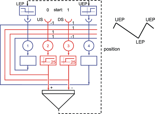
Fig. 11.9 (a) A recurrent network for the control of rhythmic movement of, for example, a wing. The net contains internal and external recurrent connections. The „external" connections shown by dashed lines represent the physical properties of the environment. Two motor units US (upstroke) and DS (downstroke) move the wing. The Heaviside characteristic has a threshold of 0.25 in both units. An integrator is used to represent the transformation from motor output to wing position. Two sensory units (blue) monitor whether the lower extreme position (LEP) or the upper extreme position (UEP) is reached. These can be represented by thresholds of -10 and 10, for example. The activation functions of neuroids 1 and 4 are linear. These sensory units have only feedforward connections with the motor units (red). The latter show positive feedback which stabilizes the ongoing activity
To conclude this section, a final remark should be made concerning the properties of systems with feedback. As already mentioned in Part I - Chapter 8 , even systems with negative feedback can show instability. If we consider a linear system with positive feedback and a nonzero input, its output will increase infinitely with time. If the loop contains an integrator the same happens, even if the input is set to zero, after some time. This can be avoided by using a limiting nonlinear characteristic, as for example the saturation characteristic. Such positive feedback plays an important role in cooperative behavior, as is found, for example, in ant colonies ( Deneubourg and Goss 1989 , Beckers et al. 1992 , Camazine et al 2003 ). Instead of a nonlinear characteristic, the use of high-pass filtered positive feedback was proposed ( Cruse et al., 1995 ). In this case the output values are not confined to a fixed range.
A special property can come into play when nonmonotonous characteristics exist, as is shown in the following example. Let us assume that we have a simple system consisting of one neuroid with the nonlinear activation function described by y = a1 x - a2 x2 (a1 > 1, a2 > 0) in the loop (Fig. 11.10a). This represents a parabola and, therefore, a nonmonotonous function. Let us further assume that the input is nonzero only for a short period. In this case, the output variable approaches a stable value (a2/(a1 - 1)), if a1 < 3 (Fig. 11.10b). The output oscillates between two values for 3 < a1 < 3.44 with a period of 2 time steps (Fig. 11.10c); it shows more complicated periodicity for 3.45 < a1 < 3.57 and exerts chaotic behavior for a1 >3.57 (Fig. 11.10d). Thus, even in this relatively simple case, a feedback system is shown to have highly undesirable properties, unless some kind of random generator is actually required. As this “chaotic” behavior can exactly be computed, it is usually called “deterministic chaos”. The behavior of such a system can be characterized by a “chaotic attractor”. The most interesting property such chaotic systems is the following. A small disturbance produces small immediate effects. However, in the long run the effect of even the smallest disturbance will be dramatic (this is eventually called “butterfly effect”). As small disturbances cannot be avoided in a realistic system, any physically realized chaotic system has nondeterministic properties. As long as the disturbances are not too large, the system remains within its chaotic attractor. Weather dynamics is a familiar example.
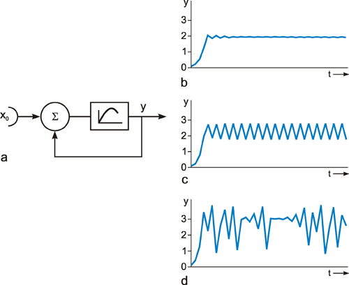
Fig. 11.10 A recurrent system can show chaotic behavior. (a) The system containing a nonlinear characteristic of the form y = a1x - a2 x2 .(b - d) Temporal behavior of the system for different parameters of the nonlinear characteristic. (b) a1 = 2.5, (c) a1 = 3.2, (d) a1 = 3.8. a2 is 0.2 and the starting value x0 = 0.1 for all cases
In contrast to feedforward networks, recurrent nets show dynamic, i. e., time varying properties as do e. g., temporal filters. This is particularly due for systems with nonsymmetrical weight distributions. For nonlinear characteristics such systems might also show chaotic behavior.
Spatial Integrator
A solution for the task of mathematically integrating an incoming signal has been shown in Part I – Chapter 4.8 . However, if this task had to be solved by real neurons, because of their limited resolution (see Part I – Chapter 8.7 ) only a limited accuracy is possible. Astonishingly, such integrations are performed, for example in navigation of ants, by an exactness of less than 1 %. How is this possible?
Assume that the system should determine the position of a limb, and that it obtains as input the speed of movement of the limb. The speed is registered by two directional sensitive sensors, one measuring movement in one direction (s+), the other measuring the movement in the opposite direction (s-). Integration of the sum of both signals provides the position of the limb. Hartmann and Wehner (1995) proposed to integrate these signals by using a spatially distributed system. In this architecture, the neuroids forming the integrator are ordered along a linear chain (Fig. B6.1). There is an input neuroid s+ at one end of the chain and a second input neuroid s- at the other end.
The system is built of simple on-off units, i. e., neuroids with Heaviside activation functions. It is further assumed that the velocity signals are coded in the form of impulses similar to spiking neurons. Therefore, a high positive speed means that in many time units neuroid s+ is excited, whereas, for a low positive speed, the probability of s+ being excited is small. Each neuroid of the chain is self-excitatory (not shown), i. e., if it was excited once and no further inhibitory influences occur, it will remain excited. What are the connections between these neuroids? Each neuroid of the chain inhibits both direct neighbors. The neuroids can be excited by both sensory units. These excitatory connections are stronger than the inhibitory ones, such that the inhibitory effect is overridden by an excitatory input signal. Finally, the excitatory input is gated by an input from the left neighbor for the s+ neuroid and, correspondingly, from the right neighbor for the s- unit (illustrated by the multiplication symbols).
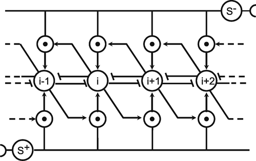
Fig. B 6.1 A simple network for spatial integration. The input unit s+ monitors the movement in one direction, the unit s- that in the opposite direction. By excitation of s+, the position of the excited neuroid of the chain is moved to the right, whereas it is shifted to the left, if s- is excited. Therefore, the position of the excited neuroid represents the integral of the input signal s
How does this system work? Assume that, at the beginning, the i-th neuroid of the chain is already excited (this corresponds to setting the value of the integrator at time t0). If an excitatory input arrives, say from the s+ unit, the right neighbor, neuroid i + 1, will be excited, and the excitation of neuroid i will, as a consequence, be suppressed. If another impulse from s+ arrives, again the next neighbor to the right, neuroid i + 2, will be excited and it will, in turn, inhibit neuroid i + 1, its left neighbor. Thus, every impulse from the s+ unit shifts the activity peak of the chain by one unit further to the right. If, on the other hand, the limb is moved in the opposite direction, the s- unit will be excited and, correspondingly, the excitation peak will be shifted to the left. Thus, the position of the peak on the chain represents the limb position and, therefore, the result of the integration of the velocity inputs.
A particular advantage of this architecture using "moving activity patterns" is that it can also be easily used to represent cyclic variables as e. g. angular values. This can be done by simply connecting both ends of the chain to form a circle ( Hartmann and Wehner 1995 ). In this case, the problem usually occurring when cyclic variables have to be treated by analog values is solved naturally. The precision of such a distributed integrator could be increased by increasing the number of units in the chain. Furthermore, application of the coarse coding principle ( Chapter 10.1 ) may be another way of improving the resolution of this system.
We have so far dealt with the properties of nets whose weights were assumed as given. One important question, of course, is how to find those weight values that ensure that the net is endowed with the desired properties. Below the six most important methods of how to set the weights are given.
In the learning matrix (Fig. 10.7) it could be seen that the weights of each output neuroid correspond exactly to the excitation of their input patterns. How could this weight distribution have been obtained? This can be done as follows: We use the schema of the learning matrix without the subsequent winner-take-all net. We apply the input pattern x as usual, but give the desired output pattern y directly on the output units (training vector in Figure 12.1a). The weights can then be obtained according to the rule wij = xj yi. This means that the weight is a result of the product of the excitations of the two neuroids involved in the connection. This is in accordance with the learning rule, theoretically postulated by Hebb in 1949 , in which the strength of a synapse is assumed to increase when the presynaptic and postsynaptic membranes are simultaneously highly excited. The strength of the synapse does not increase, however, if only one of the two neurons is excited. As a simple example, the Hebb rule might be the basis of classical conditioning or Pavlovian learning (Fig. 12.1b). Assume that a connection w1 > 0 exists between the input (unconditioned stimulus, UCS) and the reaction R to form a reflex. The weight between a second input (conditioned stimulus, CS) and the output is assumed to be w2 = 0 at the outset. If the two input signals UCS and CS occur simultaneously, according to the Hebb rule, w2 increases such that the conditioned stimulus alone can elicit the response R.
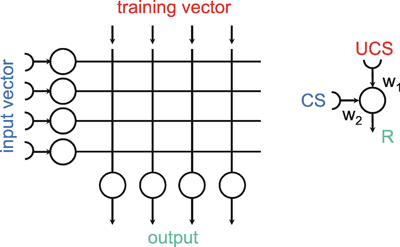
Fig. 12.1 The weights of a network can be changed according to Hebb's rule, if input vector and training vector (the desired output) are given simultaneously to the net. This corresponds to the Pavlovian type of learning (or classical conditioning) of a conditioned reflex (b). At the beginning, the weight w1 > 0 connects the unconditioned stimulus (UCS) with a reflex response (R). When the conditioned stimulus (CS) is given simultaneously with UCS, according to Hebb's rule the weight w2 being zero at the beginning increases and a conditioned reflex is activated
In most cases it is useful to change the weights not in one learning step, but in several smaller steps. Hebb's rule then runs as follows:

in which the ε parameter, which is called learning rate and takes a value between 0 and 1, determines the step size of the "learning process". If several patterns are to be stored in the same net (Fig. 12.1a), the different patterns can be applied successively at the input, and the weights are changed according to Hebb's rule.
If all components of the training vector but one are zero, as was the case in the example of Figure 10.7, each neuroid of the output layer "learns" the weights belonging to one input pattern (that one for which is shows a non zero output). If, in the general case, all components of the output vectors may be different from zero, this learning procedure produces some "crosstalk," i. e., the weights of each neuroid are influenced by all other training vectors. Under what conditions can we obtain a weight distribution which permits several input - output patterns to be stored, i. e., so that after the learning phase is finished, each of these input vectors produces its corresponding output vector without error? With the aid of Hebb's rule, the only patterns that can be stored without "crosstalk" are orthogonal to each other. This means that the scalar product of each pair of input vectors is zero. A simple case of orthogonality is given, for instance, when, in a net of n neuroids, each of the maximally n patterns is characterized by the fact that one neuroid takes value 1 and all others take value zero (see the example given in Figure 12.2a).
A disadvantage of Hebb's rule is that, during prolonged learning, the absolute values of the weights tend to increase. This can be avoided either by assuming that, according to a proposal by Grossberg (see Hertz et al. 1991 ), the sum of all weights of a neuroid must not exceed a maximum upper limit (which may be a plausible assumption in biological terms, after all) or that all weight changes are superimposed exponential decrease. This would mean that a weight that is rarely increased takes a lower final absolute value than a weight that is continuously growing during learning.
With the help of this method, Hebb's rule can be applied to feedforward nets to produce a heteroassociator. Hebb's rule can also be used for the training of a Hopfield net (Fig. 11.5) and, in this way, for producing an autoassociator. The Hopfield net is endowed with the properties of error correction, as described earlier, because all neuroids of a pattern which exhibits the same sign at the output are mutually linked with each other via positive weights. Those neuroids exhibiting different signs at the output are linked via negative weights. This has the effect that, when applying only a part of the complete input pattern, the remaining neuroids are excited via these weights in the same way, so that, after only a few iteration cycles, the entire pattern can be completed. How can the weights be adjusted so as to fulfill exactly the conditions mentioned? Here, too, these conditions are met, if the synaptic weight results from the product of the excitation of the two corresponding neuroids. This can be achieved in the following way: at the input of a Hopfield net that pattern is presented for which the weights are to be adjusted. If, starting with randomly distributed weight values, the weights are changed according to Hebb's rule, two neuroids with negative excitation as well as two neuroids that are positively stimulated, will be linked with positive weight values, while the neuroids that exhibit different signs are coupled with negative weights. In this case, too, the modification of weights is carried out not in one, but several small steps. The weight between neuroid i and neuroid j at the moment of t + 1 is thus calculated such that wij(t + 1) = wij(t) + ε yi yj. From this follows that symmetrical weights (wij = wji) result for the Hopfield net.
An attractive property of Hebb’s rule is that it can be interpreted on a local level, because the weight changes due to the strength of the “presynaptic” excitation (Fig. 12.1b, neuron CS) and of the “postsynaptic” excitation (Fig. 12.1b, neuron R which is excited via neuron UCS). Actually there are biological mechanisms known that correspond to this principle ( Kandel et al. 2000 ). However, there is also a problem, if one wants to apply this mechanisms directly to a classical conditioning procedure. Assume that there was already some learning such that weight w2 > 0. If now only the CS was presented several times, the weight w2 would further increase because both neuron CS and neuron R are excited. This property has been termed “runaway effect” by Sejnowski and Tesauro (1989) . This effect is, however, in contrast to what happens in the corresponding biological experiment. Presentation of only the CS without an UCS would lead to extinction, i.e. a decrease of the reaction R.
By means of the Hebb rule a two-layered feedforward network can be trained to store different pairs of input - output patterns. To avoid crosstalk between the different patterns, the input vectors have to be orthogonal. The Hebb rule can also be applied to recurrent networks to produce an autoassociator.
If Hebb's rule is applied to a Hopfield net, the mere input of the input vector is sufficient: if a feedforward net is to be trained, the output pattern needs to be given in addition. For this reason, this process is also called supervised learning. One alternative way of training the weights of a net (whether a feedforward net or, as described later, a recurrent net) to produce a given output pattern is to use the so-called delta or Widrow-Hoff rule. First, the input pattern x is presented. The corresponding output vector y is then compared to the desired output vector (or training vector) t by forming the difference δI = (ti - yi) for each component yi. The weight between the i-th input neuroid and j-th output neuroid is then changed according to

The change of the weight is thus determined by the magnitude and sign of the "error" (δ I = ti - yi).The change also depends on the magnitude of the input signal xj If the value of the input signal is near zero, the corresponding weight barely changes. In contrast to Hebb's rule, the change in weight ceases, once the value of the training vector has been attained.
Which properties can be imprinted upon a net with the aid of the delta rule? If only a neuroid is considered, whose activation function represents a Heaviside characteristic, the Perceptron-Convergence Theorem states the following ( Minsky and Papert 1969 ): If a weight distribution can be found by which the total number of trained input patterns can be divided into two groups, so that the input patterns of one group produce a subthreshold output value, and those of the other group a suprathreshold output value at the neuroid considered, a corresponding weight distribution can actually be obtained with the delta rule in a finite number of learning steps. Such a division into two groups is possible if the two sets of patterns are linearly separable (see Chapter 10.7 ).
If, instead of a single output, the entire net with n input neuroids and m output neuroids is considered, the question arises as to what kinds of input patterns are needed to ensure that they can be stored in the net simultaneously without influencing each other. In contrast to Hebb's rule, which can be used only to store orthogonal patterns, the restrictions applying to the use of the delta rule are less rigorous; with the latter, patterns can be stored without overlap, if they are linearly independent. The maximum number of patterns to be stored does not increase, however. For n neuroids, there are maximally n linearly independent patterns. (If Heaviside characteristics are used, this figure is higher, i. e., maximally 2 n). Examples of orthogonal and linearly independent patterns are given in Figures 12.2a, b.
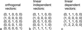
Fig. 12.2 Examples of five orthogonal vectors (a), five linear independent vectors (b), and four linear dependent vectors (c)
As shown with the simple example of the learning matrix, the adjustment of the offset or threshold values can be very important if a specific behavior of the net is to be obtained. The size of the offset of the neuroid can also be learned by using a simple trick with the help of the learning rules discussed here, although, strictly speaking, they can only change weights. For this purpose a so-called "bias neuroid" is introduced. It is not given an input and exhibits the constant excitation 1. It is linked to all neuroids of the net. The corresponding weights can, of course, also be adjusted by applying the learning rules. The bias neuroid has the effect that for each neuroid the value of the corresponding weight is added. This effect is the same as if the offset of the activation function was shifted. If this is a threshold, it would represent a shift in the threshold value.
The delta rule can also be used to train recurrent nets. For this, one iteration cycle is performed after presentation of the input pattern; subsequently, the results are compared with the training pattern and the delta rule is applied. The operation will be successful, if the desired mapping is "legal," i, e., if the condition of linear separability is given for each neuroid at the output. (If this condition is not met, the mapping can be legalized by an introduction of additional neuroids, as described above in relation to the introduction of hidden layers ( Levin 1990 )). In this way, a recurrent net can also be employed as a heteroassociator. The net shown in Figure 11.9 was obtained in this way. This shows that, with the help of the delta rule, it is possible to obtain recurrent nets with asymmetrically distributed weights.
Using the delta rule, a two-layered feedforward network or a recurrent network can be trained. The growing of the weights is limited. The input vectors have to be linearly independent to avoid mutual influences. The introduction of a bias neuroid permits the training of threshold values.
In feedforward nets, the application of the delta rule is restricted to two-layered nets. The study of highly parallel systems has been considerably accelerated by the development of methods that can be employed to train multilayered feedforward nets. This method, known as the generalized delta rule or error back propagation, merely presupposes that the activation function f(u) of the neuroids are differentiable. This excludes characteristics with discontinuous slopes like the Heaviside function. But the latter can, of course, be approximated by the frequently used sigmoid (or logistic, or Fermi-) function f(u)= 1/(1 + e-ax). To begin with, as with the delta rule, the error δ i = (ti – yi) is determined for each neuroid after the response to an input pattern has been determined. This error is then multiplied by the derivative of the value of the activation function f’(ui). Similarly to the delta rule, the weights of the neuroids of the output layer change such that

For neuroids of the higher layers, the δ error is computed as the sum of all weighted errors of the following neuroids. With respect to the weight w42, i.e., the weight between neuroid 2 and 4 in Figure 12.3, this means:

The error is thus computed back across the net (error back propagation). Therefore, the change of the weight w42 is determined by

The logistic function y = f(u) is usually used, because it is endowed with an easy-to-compute derivative: y' = y(1 - y). Although this was not specifically mentioned, the logistic function was applied in the network of Figure 10.9b. Unlike the simple delta rule, with the help of the generalized delta rule, even those patterns can be learned which are linearly dependent (see Figure 12.2c for an example of linearly dependent patterns).
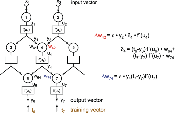
Fig. 12 .3 A simple, three-layer network for the illustration of the generalized delta rule. As examples, the formulae of how to change weights w42 and w74 during learning are given
The properties of the delta rule can be illustrated as follows. For a given pair of input and training patterns, the total error produced by a given weight distribution can be defined as
 ,
,
i. e., the sum of the squares of all errors produced by all output units. The aim of the learning procedure is to minimize this error value. As the error depends on the values of all k weights, the situation can be described as a function in a k-dimensional space. The goal is to find the minimum of the error function in this k-dimensional space. The delta rule is a gradient descent procedure. The gradient descent changes the weights in such away that the error is continuously reduced. The procedure starts at a position in the k-dimensional space given by randomly chosen initial values of the weights. During this gradient descent, there is, of course, a risk that the procedure gets stuck in a local minimum so that the optimum learning performance is not realized. This risk can be reduced by increasing the number of hidden units. This increases the dimension of the space and will in turn reduce the incidence of local minima because the introduction of an additional dimension may open a way out of the minimum. A further method consists in superimposing random values on the weights during the learning process. This can provide the possibility of moving against the gradient and thus to overcome local minima; during training the amplitude of this noise should continually decrease. This procedure is eventually called simulated annealing.
Another simple and often used method is the introduction of the momentum

This means the direction of descent does not only depend on the actual gradient but also to some extent, given by the factor η, on the direction and size of the last step. Thus, some kind of low-pass filter-like inertia is introduced which might also help to avoid local minima.
The time to approach the minimum can be shortened by application of the RPROP algorithm ( Riedmiller and Braun 1993 ): for each weight, the amount of the weight change increases by a given factor, if the gradient does not change its sign. If, however, the gradient has changed its sign, which means that the learning algorithm has just jumped over a minimum, the weight change is decreased by a given factor and its sign is changed, too.
To illustrate why the generalized delta rule requires a differentiable activation function, we have to consider the error function as a function of the weights. Considering weight w74 in Figure 12.3 as a simple example, the error function is defined as E(w74) = (t7 – y7)2 = (t7 – f(u7))2 = (t7 – f(y4 w74))2. Calculation of the gradient means to determine the first derivative of E with respect to the weights. According to the chain rule, we obtain

If the logistic or a similar function is used, the derivative has the property of being near zero for very small and very high input values, but high for values around the middle range. This could be interpreted as the weights do not change if the unit has "decided" to assume a very high or very low excitation, whereas learning is more probable as long as no such decision yet has been made.
Whereas the number of input and output units is given by the task for which the network is designed, it is an open question how many hidden units should be used. Generally, a given mapping can be approximated better, the more hidden units exist in the net. On the other hand, however, too many hidden units destroy the capability of generalization; the net learns the exact training patterns only and may not appropriately respond to other, though similar input patterns. This is called "overtraining, or overfitting." It is still an unsolved question what structure of a network (number of units in a layer, number of layers) is best suited for a given problem. One method to improve, i.e., simplify, the structure of a network, which has already been shown to solve the required task, is to look for those neuroids which have the smallest weight values, delete them and try to retrain this new network with the same task. By this "pruning," one may find a simpler version of the network. (For alternative methods, see Chapter 12.5 ).
Finally, it should be mentioned that the generalized delta rule can also be used for recurrent nets, as discussed above in connection with the simple delta rule. However, there is the problem that the dynamics of the recurrent net as such are superimposed to the dynamics due to the weight changes during learning. This problem is avoided by “unfolding” the recurrent network into several identical feedforward nets (Fig. 12.4). Each net in the spatial order corresponds to another iteration in time (“unfolding in time”). This means that the backpropagation method can be applied in such a way that, after having given the input to the uppermost net, the output of each net in the series has to be compared with the desired output expected in the corresponding time slot (backpropagation through time, BBTT, Rumelhart et al., 1986 ). All errors for a given weight are collected and used to train this weight (for details see Hertz et al. 1991 ). Different to the backpropagation method applied to feedforward networks, BBTT by itself may show complex dynamic behavior and does not necessarily lead to a minimum.
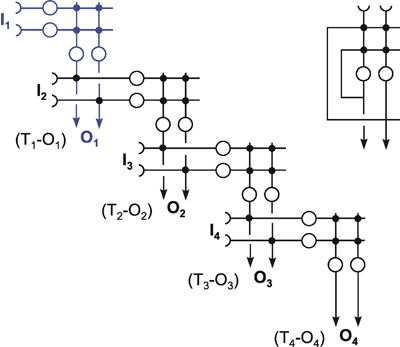
Fig. 12.4 Unfolding a recurrent network in time. To cope with the dynamics of a recurrent network, the net is copied several times, and these copies are connected to form a feedforward net. Each subnet represents another time step. Errors (Ti-Oi) have to be collected for each time step, i.e. for each subnet, and are then used to update the weights
To train networks with more than two layers, the generalized delta rule or error back propagation can be used. This requires differentiable activation functions. Crosstalk can be avoided also for linear dependent input vectors. Several methods are available to avoid getting stuck in a local minimum during the learning process. How to choose the appropriate numbers of hidden units and layers is a still unresolved question.
A flaw of the generalized delta rule is that it is hard to believe that learning in biological systems is actually based on this principle. One problem being that additional networks are necessary to compute the error and transport this information to the corresponding synapses. The other problem concerns the determination of the error as such. How could the single error components be determined and provided to the backpropagation network? Furthermore, the training methods described above are used off-line, i.e. the recurrent connections are switched off during learning to avoid the problems of superimposition of two dynamics, the dynamics of the recurrent net itself and the dynamics due the changing of the weights ( Steil 1999 ). In the following a circuit is presented that copes with this problem. This circuit acts within a neuronal unit and incorporates a learning rule that formally corresponds to the delta rule, but does not require a separate network for backpropagating the error because the latter is computed locally within each single neuroid. The units, called input compensation units (IC units, Kühn et al. 2006 ) contain a circuit that allows to disconnect the dynamics of the recurrent network from the dynamics due to the learning procedure. The function will be illustrated using a simple task: The network should learn to represent a fixed static pattern given at the input to produce sustained activity even if the input pattern disappears. Specifically, the task is as follows: the net consists of n units. As example, a net of n = 3 units is depicted in Figure 12.5a. Any n-dimensional input vector a is provided to the net. The learning algorithm should change the weights in a way that all units adopt activations that correspond to the input and maintain their activation even after the external input is switched off. The task is to find a weight matrix W with a= W a. As we have n2 weights, there is a manifold of matrices that fulfill this condition. n equations determine n degrees of freedom. Therefore (n2 – n) of the n2 weights can be chosen arbitrarily. For n = 3, for example, one possible solution is given by

Such a net can also be described as forming an attractor consisting of a two-dimensional subspace that is described by the plane a1 x1 + a2 x2 + a3 x3 = 0. This net is only neutrally stable, which means that if any weight is changed arbitrarily, the activations of the units increase infinitely or decrease to zero. Therefore, a learning mechanism is necessary to stabilize the weight against disturbances.
In order to achieve this, each neuroid is equipped with two types of inputs: One external input ai, the weight of which is fixed, and n internal, i.e., recurrent input connections xj, the weights wij of which can be changed by learning. The overall output of one neuroid is calculated in the following way:

(1)
The + means that only the positive part of the expression within the bracket term is transmitted, i.e. a rectifier is applied. The structure of an Input Compensation Unit is schematically shown in Figure 12.5b.
From equation (1) it is immediately clear that the output xj of the network always equals the external input independent of the actual weight size because the sum of the weighted internal inputs si is added and subtracted instantly again. Therefore, this built-in compensation mechanism protects the global dynamics of the network from the learning dynamics. This enables us to train a recurrent neural network consisting of IC units online, i.e. without cutting the feedback connections during training.
The weights are changed according to the following algorithm:
 (2)
(2)
with ε > 0 being the learning rate and δ i(t)=ai(t)-si(t). During the training procedure, the weights stabilise at values that in the end the summed recurrent input si equals the external input ai, i.e. δ i(t)=0. After learning is completed, and the summed internal input equals the external input, the latter can be switched off without changing the activation of the net. However, learning has to be switched off, to, because otherwise the weights would learn to represent the zero vector (0,0,0).
A recurrent network consisting of such IC units (Fig. 12.5a) can be trained with any vector a, or with a number of vectors that point to a subspace of dimension < n. As there are redundant degrees of freedom, some of the weights can arbitrarily chosen. For example, the diagonal weights could be set to zero. Furthermore, any dynamic situation can be learnt that can be described by linear differential equations (see Chapter 14.3 ).
Below, two further learning procedures will be presented, which also come closer to biological reality than the classical backpropagation method, namely the reinforcement method and the method of genetic algorithms. Both start from the assumption that feedback from the environment does not mean that the correct output pattern is given and then compared to the actual output; rather, what is implied is that the environment merely supplies a scalar quantity, e. g., a value between zero and one, comparable, for instance, to a quantitative judgment of the answer varying between good and bad.
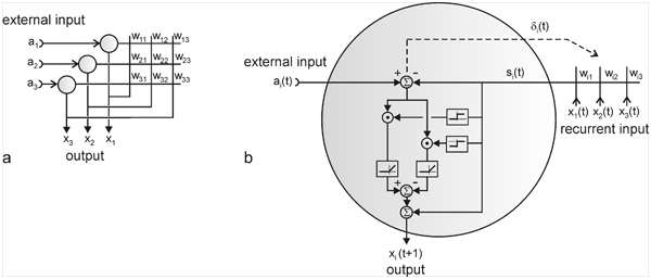
Fig. 12.5 Recurrent network with IC units. (a) A network containing 3 units. (b) The circuit characterizing an IC unit.
Application of IC units allows online training of recurrent networks because they permit to separate the dynamics of the recurrent net from the dynamics due to the weight changes.
With the exception of the autoassociator trained by Hebb's rule or the IC algorithm, the net has so far always been informed of what the correct answer should be. In this context, learning is based on the evaluation of the difference between the response of the system, presented by the net to a specific input vector, and the actually correct answer, given by the trainer. Thus, an error signal can be determined for each component. These methods are described as supervised learning. Most often, however, an organism is not informed of the right answer in a specific case, and feedback merely consists of a scalar quantity (e. g., on a scale good-bad). If a ball is thrown at a target, for example, there is no feedback on the correct control of individual muscles, only on whether it hit or missed the target. This would be a case for reinforcement learning. Since feedback to the system consists only of information about whether the action was good or bad, but not about what the correct action would have been, we talk of a critic here, rather than of a trainer. In a simple case, the feedback is immediately provided by the environment. The more complicated case, when the feedback occurs only after several actions have been performed, will be treated later.
The input components xi, describing the external situation, and the components of the output vector y may be positive real numbers (Fig. 12.6a), although in many examples, the neuroids of the output layer are endowed with a Heaviside activation function and can take the values 0 or 1. The system is presented with a number of input vectors. The task is to learn reactions to these inputs that will be rewarded as highly as possible. The net initially possesses a random distribution of the weights wij, and hence responds to an input excitation by reaction y, which is presumably not very sensible. The environment ("world") evaluates the system's reaction and responds by giving a reward r. The aim is that the weights wij within the systems should be changed in such a way that the reward r for the various input vectors is as high as possible (this corresponds to the situation in which the extreme value of a quantity has to be found.)
This task can be split into two problems, namely, first, to find an action y which provides a high reward, and, second, to find the weights for which, for a given input x, i.e. a given situation, the system produces the output y. The latter corresponds to the paradigm of supervised learning and, therefore, can be solved as described above by application of the delta rule or, if the activation functions are differentiable, e. g. logistic functions, by the generalized delta rule. The first task is the actual problem of reinforcement learning.
To begin with the simplest case, we assume that the world behaves deterministically. This means that a definite change of the action produces a predictable change in the reward. Let us further assume that the same input vector is presented several times in a row, i. e., that the environmental situation remains unchanged. The change in reward can then be compared for two successive actions. At moment t - 1, the system is informed of input x(t - 1), reacts by y(t - 1), and receives reward r(t - 1). A corresponding situation occurs at moment t. In order to search for a better action, yi(t) is changed compared to yi (t - 1) by means of an addition of noise. The effect of this changed action can be quantified by multiplying it with the change in reward:

This value Δyi can then be used to solve the second task, namely to calculate the weight changes of the net. If this net contains several layers, the generalized delta rule can be applied. To simplify matters, it will be shown here for a two-layered net:
 (see
Chapter 12.3
).
Δyi thus corresponds to the error signal of the delta rule. For a linear activation function, this means

The net can then be trained by changing the weights in the following way (see Fig. 12.6) ( Barto Sutton Brouwer 1981 ):

On the basis of this learning rule, weight wij changes only if the activity of neuroid i changes, i. e., Δyi = yi(t) - yi(t -1) ≠ 0, and if the reward changes. The weight increases if the state of activity and the corresponding reward change in the same way. Otherwise the weight decreases. As a consequence, the rewarded behavior will follow this input vector with greater probability. If we introduce Heaviside activation functions, only the sign of the difference yi(t) - yi(t - 1) needs to be used in equation (1) in order to obtain a Δyi of ± 1 or 0.
Stochastic properties might occur in the world such that the reward is noisy. In this case, a direct comparison with the action and the reward at time t - 1 may not be as good. Instead, the comparison with the mean values of earlier actions and rewards can lead to greater improvement of the weights.
In some particular cases, it may happen that r is scaled in such a way that a baseline or reference value ro (e.g., = 0) can be given so that above ro, r can be considered a positive reward and below it, a negative reward. The value (r - ro) then has the property of being a positive or a negative number. In this case, the comparison with the baseline value is possible, of course, and actually leads to faster learning ( Williams 1992 ).
In principle, the reinforcement learning procedure corresponds to the operand conditioning (or instrumental learning) found in biological experiments. A rat in a Skinner box accidentally (see "noise" in Figure 12.6a) performs an act e. g., pushes a lever. If the lever is connected to a rewarding mechanism, there is greater probability that this behavior will be performed again.
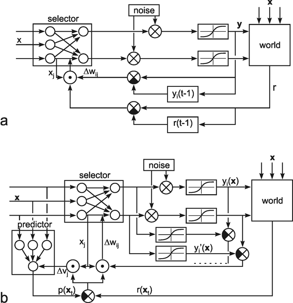
Fig. 12.6 Reinforcement learning. (a) The input vector x is given to the network, which, in this example, consists of two layers, but might be more complicated. The response of the net is somewhat changed by means of a noise produced by the system. The system contains a memory to store the components of the output vector applied during the previous time step [yi(t-1)]. Furthermore, the system receives a scalar reward signal from the environment (world) and stores the previous reward value r(t-1). With these values, the appropriate change of the weights wij can be determined as shown in the lower part of the diagram. (b) If the input vector varies, the application of an additional "predictor net" can solve the problem. In this case, the actual reward is compared with the expected reward p provided by the predictor net. Here, the output vector is not compared with the previous one, but with the original vector that the network proposed before the vector was changed by means of the noise influence. These values can be used to change the weights of the selector net and of the predictor net, accordingly.
This disadvantage of the method described above is that it presupposes that the input vector (i.e., the environment) does not change or, if it does, perhaps just a little. In case of a sudden change, a comparison with the preceding situation would indeed not make much sense. In such a situation, a different reward is attributed to an action y depending on the input vector x. To solve this problem, an additional net is introduced which provides the reward to be expected for a given input according to the earlier experience. This net is called predictor net because it provides the predicted reward p(x) for a given input x (Fig. 12.6b). If we had an ideal predictor, the value r(x t) could be compared with the value p belonging to a given input vector. How can we obtain this net? The predictor net comprises a simple world model, so to speak, which computes the reward to be expected in connection with a specific input signal by p(x t)=Σ vj xj(t), vi being the weights of the net. This predictor net is simple to train since the reward p predicted by the predictor net can be compared to the actual reward r, thus enabling a direct application of the delta rule:

If a multilayered predictor net is used, the generalized delta rule could be applied accordingly.
Using the predictor net, the synapses of the net itself, sometimes called the selector net, can be trained, as above:

y’ is the action proposed by the selector. It is not possible to train only the predictor net because the reward depends on the actions y. Therefore, both nets have to be trained in parallel. The better the predictor net becomes in the course of learning, the smaller the error (r - p) will be, such that the predictor net, and thus the net itself, will move toward a stable final state.
In the simple version illustrated by equation (1) the system requires a storage for the earlier reward r(t - 1) and for the components of the earlier action yi(t-1). Thus, if the output vector has n components, storage for n + 1 values is necessary, which stores the information from the last time step. By contrast, the system described by equation (2) and Figure 12.6b requires no such storage.
TD learning: Where the net acts in a deterministic world, i. e., a world that responds to a particular reaction y of the net with a particular environmental situation x, time series can also be learned in the same way. Pure reinforcement learning can, however, only function in a simple world. But a case may arise in which, in a specific situation x, a reaction y may be reinforced (and hence learned) even though the system, through action x, is confronted with a situation in which it may be difficult to perform new, reinforced actions. For example, if an animal eats up all available food, this may be desirable for the moment. But a decision to exercise temporary restraint may be preferable in the long term, since this might possibly prevent starvation. It would be better, therefore, instead of a momentary reinforcement r (t), to consider the reinforcement r∞(t), which represents a combination of all further reinforcements to be obtained in this series of actions. In order to include to long-term effects of actions, TD (temporal difference) methods have been introduced by Barto et al. (1981) (Fig. 12.7). Assume that for each situation (input x) a number of actions are possible. The selector net chooses one of these actions. The function y = f(x), which describes which action is selected for a given situation, is called the policy or strategy of the system and is represented by the properties of the selector net. The reward r(t) depends on the situation x t and the action y t = f(x t) chosen, and is therefore written as r(x t, y t). As actions in the far future may be less important, for example, because they can be less exactly foreseen, they are given smaller weights. Barto et al. proposed to determine

with γ < 1 which produces smaller weights for more distant rewards. This can also be written as

Equations (3) hold for an unpredictable world, i. e., the reward may be influenced by noise and so may be the reaction of the world, namely the new input x t + 1. In order to find a good strategy, in the TD reinforcement approach, the predictor net is replaced by an "evaluator net." For each action, this provides an estimate e(x) for the value r∞(x). The problem now is hot to learn a sensible evaluator net which can produce the value e(x), for a series of actions. Although the selector proposes action y', a new action y(x t) will be tested by means of a new input. This leads to the reward r(x t). If this reward is better than that expected for action y', the evaluator net should be changed. According to the earlier case (reinforcement comparison, equation 2), this would be done by directly comparing the reward r(x t) with the predicted reward p(x t). As in TD learning future rewards should also be taken into account, so the expected value includes not only the actual reward r(x t), but also the (weighted) rewards expected in future consecutive actions. As the expectation value e is an approximation to r∞(t), equation (3) holds approximately also for e:

Thus, e(x t) should not be compared with the actual reward r(x t), but with the complete exceptation r(x t) + γ e(x t+1). This leads to an "error" signal

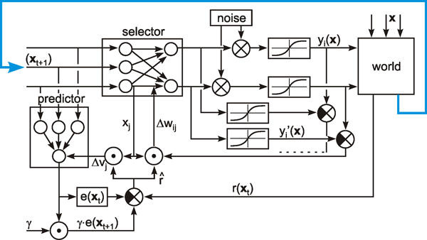
Fig. 12.7 Reinforcement learning. Temporal difference (TD) reinforcement permits finding a temporal chain of actions such that the total reward obtained during the complete chain is used as the criterion rather than the possibility high reward of an individual action. In this case, an evaluator net provides an estimation e(x) of the expected total reward. Using the actual reward r(x t), the expected value e(x t) and the expected value for the subsequent input vector e(x t+1), the appropriate changes of the weights of the selector net and the evaluator net can be calculated. For this purpose, as in Fig. 12.6b, the actual noisy output values are compared with the original values provided by the selector net. The uppermost bold arrow indicates that because of some physical properties of the world, an action y in a given situation x(t) leads to a new situation x(t + 1) which represents the new input vector
The value e(x
t+1) can be obtained by observing the state of the world after action y
t has been performed. This state is represented in the form of the subsequent input vector x
t+1.Thus, the system needs to store the values r(x
t) and e(x
t) until e(x
t+1) is computed. Using
 the weights of the evaluator net can be changed according to

In this way, the evaluator net is improved. As in the other cases of reinforcement learning (equation 2 b), the signal
 can be used to train the weights of the selector net:

These procedures are schematically summarized in Figure 12.7.
If a network should be trained but detailed information concerning the output vector is not available, supervised learning methods cannot be applied. One possibility is to use reinforcement methods or learning with a critic. The critic provides only a scalar value (e.g., on a scale good-bad). Different reinforcement algorithms are used for such cases as learning a given task in a constant environment, for different tasks in a changing environment, and where long-term reward of a chain of behavior has to be evaluated.
The types of networks treated above all consist of one, unified network. When such a ”monolithic” network, that has already learnt some tasks, is trained to learn a new task, in principle all weights will be changed and therefore it is possibly that already stored knowledge may be (partially) destroyed. This could be overcome only if, during the training of the new patterns, also the old patterns are trained again. This does however not correspond to the biological situation. The problem could be solved by a modular architecture consisting of a number of independent “expert nets”, if only one of them is learning a given task. For learning n tasks we require n expert nets. ( Jacobs et al. 1991 , Jordan and Jacobs 1992) proposed to add another net, termed gating network. All n+1 nets are multilayer perceptrons (MLP) and receive the same input x (Fig. 12.8). The gating net has n outputs gi. The output vectors of the n expert nets are compared with the training vector. The overall error of each net is fed into a WTA network. Only that network with the smallest overall error, the winner, is allowed to change weights (i.e. there is a competition between the experts nets as is similarly found between single units in the case of competitive learning, see Chapter 12.8 ). This procedure guarantees that only that expert is learning that is already best suited for the actual task. In this way, the different nets specialize on different input situations. An expert for task A is not any more a good candidate to specialize on a different task B. Any one of the other nets might be better suited for the task B. The output of the WTA net is used as training signal for the gating network, too. The factors gi, being 0 or 1, are not only used during the training phase, but are also used to control the output of the experts after training. Each expert's output is multiplied by its gating factor, so that only the actual expert controls the output.
Wolpert and Kawato (1998) introduced an expansion in the way that the gating network does not receive its input from the environment, but looks at the errors produced by each expert. From these error values erri so called "responsibility" values gi are calculated which are then used in the same way as the gating values, i.e. they are used for learning and for acting. A softmax function (gi = exp(-erri 2 ) /Σ exp(-erri 2); Σgi = 1) is used that allows for a blending between several experts. This architecture has the advantage that the gating network does not have to separate all possible environmental situations.
Tani and Nolfi (1999) applied these principles to recurrent nets of Jordan type ( Chapter 14.1 ). Again, all n expert networks receive the same input. Their task is to predict the input during the next time step. All nets are trained using the prediction error (summed squared local errors) by Back Propagation through Time (BBTT; Chapter 12.3 ). Before this is done, there is a competition between the nets on the basis of the different prediction errors. Using the n prediction error values, a kind of soft winner take all circuit ("softmax function”, see above) determines a "quality factor" gi for each net. The BBTT procedure for each net is weighted using the factors gi. This means that the best network learns stronger than the other ones, giving this network an advantage in the next learning step for this situation (similar to the feature maps, see Chapter 13 , but instead of geometrical neighborhood we have here "performance neighborhood"). The quality or "gaiting factors" gi are updated using a kind of momentum rule to avoid abrupt changes through time.
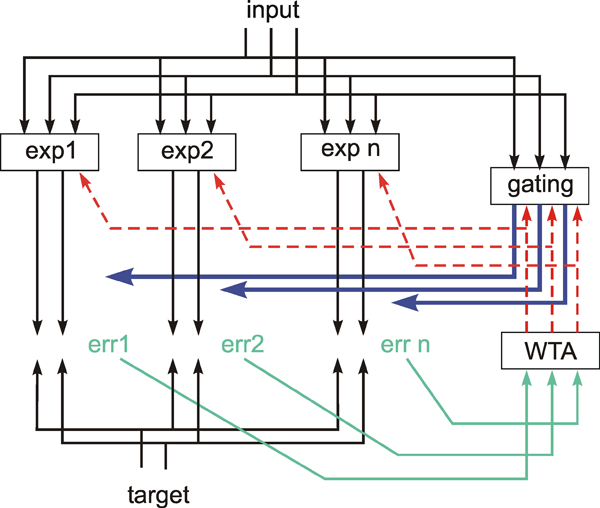
Fig. 12.8 Expert networks. N expert nets and one gating net receive the same input. The output of the gating net determines which expert has access to the overall output (blue arrows) and is used for training these experts (red arrows)
A modular architecture allows fast training of new tasks, and avoids the destruction of already acquired solutions.
While reinforcement learning corresponds to the situation that an individual net learns in the course of its "live," so to speak, the procedure of genetic algorithms or evolutionary strategies more resembles learning during the course of evolution. Each learning step corresponds to a transition from one generation of individuals to the next. The basic assumption is that there is a sizeable number of individuals (i.e., networks) that differ from each other with respect to their weight values. These nets have to fulfill the given tasks, and their quality is evaluated in terms of a one-dimensional, i, e., scalar, value ("fitness"). Subsequently, selection ensures that, in the next generation, those nets that performed relatively well during tests, occur more frequently, while the worst nets are eliminated. The nets of this new generation are now themselves subjected to mutations, i, e., weight values are varied by random influences, and this generation is then again tested. In this way, nets develop which, from one generation to the next, become increasingly well adapted to a set task. As a variation of this approach the size of random influences ("mutation rate") may decrease from one step to the next. The most important part of such a program is the choise of the fitness function or evaluation function, because the form of this function essentially determines the behavior of the algorithm.
Apart from this so-called "asexual" reproduction, the possibility of "sexual" reproduction is also being studied. In this way, a new net can be generated by mixing the weight values of two (or more) parents. With reference to biology, this is occasionally referred to as "crossing over". These genetic algorithms may also be used to search for an optimal structure for the network. For this purpose, the activations of randomly selected neuroids are set to zero and the evaluation function includes a term which counts the total number of active neuroids such that a smaller number corresponds to a higher fitness value. By this way networks that solve the task but have fewer neuroids have a better chance of surviving the selection procedure.
The comparison of this stochastic method with the gradient descent methods (the delta rule procedures) described earlier reveals that the latter are computationally faster, but suffer from higher probability of sticking in a local minimum. This is much less the case for the evolutionary strategies because the latter search in a broad range of the search space simultaneously. For more detailed information concerning the properties of genetic algorithms the reader is referred to Koza (1992) .
In a simplified version, one generation consists of only one single individual. In this case which is called random search, the fitness of the new individual is compared with that of the last one. If the fitness of the new individual is better, the new weight values are accepted. Otherwise the old weight values are maintained and another mutation is tried.
While the two learning methods described last, namely reinforcement learning and genetic algorithms, are much closer to biology than the generalized delta rule, for instance, they still have the disadvantage of requiring many more learning steps and, consequently, a computation that takes much more time than learning methods with superviser.
Genetic algorithms and random search are learning methods which do not suffer from getting stuck in a local minimum as much as gradient descent methods. However, the former are slower in general. They do not require a supervisor but depend strongly on proper selection of the evaluation function.
We have so far discussed nets in which each neuroid of one level was usually connected to each neuroid of the next level (full connectivity). Apart from the number of levels and neuroids in each level, no further structures were given. Below, we will address some nets in which only selected connections are given. In addition, the weights are divided into two types, those whose values are fixed from the beginning, and those that may change their values during learning.
The task of the perceptron with one output neuroid, as mentioned in Chapter 10.6 , consisted of dividing a large number of input patterns (input vectors) into two groups, such that a pattern of one group is responded to by 1, and a pattern of the other group by 0. This was learned with the help of the delta rule via a trainer. We will now consider a similar system which is modified in such away that two output elements are present, in which one neuroid (A) responds to the patterns of one group, with a value of +1 and the other neuroid (B) responds to the patterns of the other group by the output value +1. In this case, what should be learned is that either one or the other output element responds by 1.This can be achieved - even without a trainer - by connecting these two output neuroids by mutual inhibition, so that they represent a small recurrent winner-take-all net. This means that, starting with random input weights, one neuroid will "win," when a given input pattern is used. We can also apply a second input pattern which excites the second output neuroid more than the first. Using this pattern, the second output neuroid will win. The excitation at the output, i. e., the excitation of the neuroids after passing through the winner-take-all net, is used to train the input connections according to Hebb's rule. Then the weights of the two output neuroids, if only these two patterns are used, will be changed in such a way that the weights of the two neuroids resemble the two input patterns, respectively (except for a factor). This means the system adapts by itself, i. e., without the trainer, to the two patterns. When the weight vectors correspond to the input vectors, as illustrated in the example of Figure 12.9a (the winner-take-all net is not shown), unit A responds strongest to input i 1 and unit B to input i 2. If the net is confronted with new patterns, these are divided into two categories, depending on their similarity to either of the two original training patterns. If learning is continued when presenting the two groups of patterns, the weights of the two output neuroids adapt to some kind of mean vector of both groups. The weight vectors find clusters in the input vectors. The vector which represents the center of such a cluster can be considered the representative or prototype of this group. In other words, the net develops a "concept" of the two types of the vectors obtained from the outer world. Thus, this is called competitive learning and is a type of unsupervised learning that has the advantage that the learning phase can continue during the active phase of the system. A separation between two states, learning and operation, is not necessary as it is in the case, for example, of the delta rule.
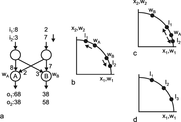
Fig. 12.9 (a) Competitive learning. A network consisting of two layers. For the given weights the input vector i 1 yields the output vector o 1 and i 2 yields the output vector o 2. The two neuroids A and B form a winner-take-all net the connections of which are not shown. Thus, neuroid A will win the competition after application of i 1 whereas neuroid B will win when i 2 presented. This means that, in the first case, only neuroid A will learn, i. e., change its weight, and in the second case only neuroid B will learn. (b) Graphical illustration of the two normalized input vectors i 1 and i 2. The two normalized weight vectors w A and w B can be plotted in the same coordinate system. The arrows indicate the change of the weight vectors during learning. (c) As (b), but showing an inappropriate arrangement of input and weight vectors. In this situation, neuroid A will win the competition for both input vectors i 1 and input vector i 2. Therefore, w A will always move between i 1 and i 2 and neuroid B will never win. (d) Three input vectors can be separated only if the second layer of the network consists of the least three neuroids
In our example, we started with two input patterns which already can be distinguished by the net. The only improvement was that during training the system finds a better representation of the two groups of input vectors. The more interesting situation, however, is to start with two given sets of input patterns and to find a net which by itself separates these two groups. As will be shown in the following, this is possible even for the more general case, where the winner-take-all net consists of more than two neuroids. The input patterns can then be divided into a correspondingly greater number of types of patterns. The net thus has the property of combining vectors into groups which are characterized by the excitation of different neuroids of the output layer. This is also known as vector quantization.
If we have n neuroids in the input layer and k neuroids in the output layer, the application of Hebb's rule (Δ wij = ε xi yj ; i = 1...n, j = 1 ... k) means that the weight vector of the winner becomes similar to the input vector x. The learning rule only works for the winner, since only here the output value yj is 1, whereas for the other neuroids it is always 0. The value of ε (learning rate) may decrease during the course of learning. The disadvantage, that with Hebb's rule weights can grow without limit, can be counteracted if the weight vectors are normalized after each learning step. (Normalization usually means that all components of the vector are multipled by a common factor such that the vector length is 1). More important, the normalization avoids one weight vector becoming so large that it wins for every input vector so that other output neuroids have no chance to learn. Assume for example, that the weights of the neuroid A in Figure 12.9a had twice their values, then the output of A and B was 136 and 38, respectively, to input i 1 and 76 and 58 to input i 2. So in each case unit A will win and unit B will never have the chance to learn. On the other hand, the disadvantage of normalization is that the effective dimension of the input vector is n - 1, and that the input space is limited. For example, if the net contains two input neuroids, not the complete two-dimensional space is used as input but only those vectors which point on the unit circle. Thus, the effective input space is only one-dimensional and is of limited extension. For three-dimensional input vectors the effective range is the two-dimensional surface of the unit sphere.
Another method would be to use the learning rule Δ wij = ε (xi - wij) yj, the so-called "standard competitive learning rule." This has the effect that input vector and weight vector gradually become similar to each other, but nevertheless the vectors have to be normalized to enable discrimination. Depending on the kind of normalization, this rule may be equivalent to the application of Hebb's rule. The situation is visualized in Figure 12.9b for the simple net already shown in Figure 12.9a where the input consists of only two neuroids. Then both the input vectors and the weight vectors can be plotted in the same plane. Because of normalization all vectors point on the unit circle. With the starting situation given in Figure 12.9b, the weight vectors w A will be pulled to the input vectors i 1 and w B to i 2. However, there is still the problem that success depends critically on the distribution of randomly chosen weights at the beginning. This can be shown in Figure 12.9c where both input vectors will attract only weight vector w A. This will move to and from between i 1 and i 2 whereas the second output neuroid (vector w B) will never win and therefore never change its weights. Thus, successful learning is not possible for any arbitrary configuration of weights at the beginning. A way to avoid this problem is to start with weights that are not randomly distributed but already equal some of the input vectors. This heuristic, of course, also decreases the time needed for learning. Another solution is "learning with conscience," where those units which often win are gradually excluded from the competition, so that other "dead" units also have the change to learn.
If we want to avoid the disadvantages of normalization and the reduction of the input dimension, the following net could solve the problem. One can use the standard competition learning rule. After learning is finished, the output value of the neuroids of the second layer is not determined by computing the scalar product y = f(Σ(xiwi)), but computing the Euclidean distance between vectors x and w, according to
 .
.
For f(u) the Gaussian function often is used. Then only a neuroid the weight vector of which equals the input vector x is excited by 1. The excitation of any other neuroid decreases exponentially with the Euclidean distance between the weight vectors of both neuroids. Neuroids of this form are called radial neuroids. However, such radial neuroids can probably not be realized by a single biological neuron but require a microcircuit consisting of a number of biological neurons as will be explained in the next paragraph.
The following arrangement could ensure that, with a particular input excitation, only the topologically corresponding neuroid of the second layer will respond (Fig. 12.10). The network mentioned above, consisting of a small number (e. g., k = 2) of neuroids in the input layer and n topologically arranged neuroids in the second layer, has to be expanded in the following way (in the example in Figure 12.10 we use k = 2 and n = 3). All neuroids are referred to by using their activation values as shown in Figure 12.10. The input neuroids are x1 and x2, respectively, in Figure 12.10. Each of the n neuroids of the second layer is replaced by k neuroids, here xi1 and x i2 (i = 1 to n). Each input layer neuroid x i is connected to the n neuroids x ij (i = 1 to n, j = 1 to k) of the second layer by a weight fixed to value 1. In addition, a bias neuroid, showing an excitation of - 1, is introduced which is linked to each neuroid of the second layer via variable weights w ij. (The indices in this case are identical to those of the corresponding neuroid of the second layer).
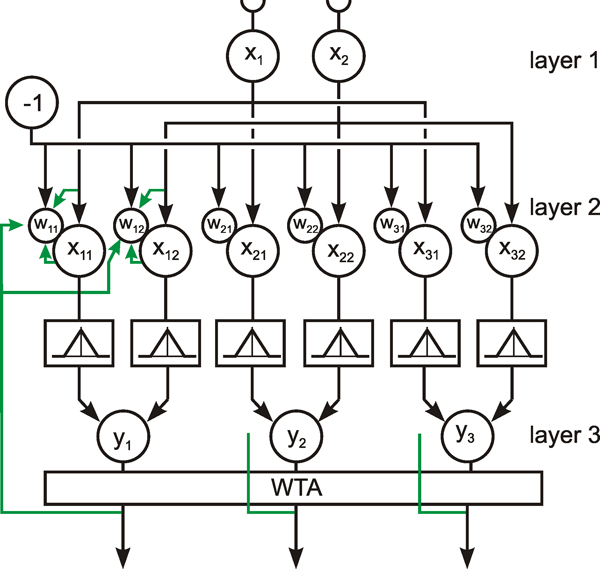
Fig. 12.10 Competitive learning without normalization. This network can learn to separate groups of vectors (in this example three) distributed over the whole two-dimensional space x1, x2. The changeable weights are shown by small circles
The output of each neuroid of layer 2 is endowed with a Λ-shaped activation function (e.g. an inverted full-wave rectifier or a Gaussian function). The outputs of the k related neuroids (xi1 to xik) are added to a further neuroid yi(i = 1 to n) of layer 3. The output of the neuroid yi corresponds to that of a radial neuroid, as it reacts maximally if (x1 - wi1)2 + (x2 – wi2)2 is zero (or in other words, the input vector and the weight vector are identical). This means that in this way a radial neuroid is described by a small network consisting of k + 1 simple neuroids. A subsequent winner-take-all network decides which of the neuroids yi is most excited. Learning is performed for neuroids xij which have the same first index i as that of the winning output neuroid yi. Learning is not applied to the synapse between input and neuroid of the second layer, but to the weights wij (j = 1 to k) of the bias neuroid. Hebbian learning is applied according to the rule wij = ε yi xij xj (j = 1 to k). This is shown by broken lines in Figure 12.10. In this way, after learning is completed, only that neuroid of layer 3 that corresponds to the input vector is given an output value of 1. All others are given a lower output excitation, which is smaller the greater the distance to the maximally stimulated neuroid.
As in earlier cases, the solution of problems which are not linearly separable (for example when input vector i 1 and i 3 in Figure 12.9d should be grouped together to excite output unit A and input vector i 2 should excite output unit B) is only possible when several such networks are connected to form a system consisting of more than two layers.
One problem of competitive learning networks is that the number of clusters into which the input vectors (patterns) should be grouped, is predetermined by the number of units existing in the output layer. If the net contains more neuroids than the types of input patterns that occur, the categorisation might be too fine. This problem was solved by the so-called ART (adaptive resonance theory) network introduced by Carpenter and Grossberg (1987) in several versions. Only the qualitative properties of this network type will be described here. The network contains a large number of output units which, at a given time, can be distinguished between being "enabled" or "disabled." Each enabled unit is responsible for a cluster of input patterns; the disabled units did not respond to one of the input vectors presented up to this time. Only when an input vector occurs which cannot be attributed to one of the units already enabled, will one of the disabled units change state and become responsible for this new category. An input vector corresponds to a "new" category if the distance to each of the already existing prototype vectors is larger than an adjustable, prespecified parameter. If this parameter is high, the input space is divided into coarse intervals, if it is small, a large number of output units may be necessary to cope with the finer resolution required. Of course, the number of possible categories is not infinite but limited by the number of available output units.
Competitive learning requires a prestructured network where only selected weights can be changed according to Hebb's rule. It provides a method whereby input vectors can be grouped without any trainer or critic, neither is the introduction of an evaluation function necessary. No switch from learning phase to action phase is necessary, rather learning can continue infinitely.
Up to now there has been no special requirement as to how the neuroids in the second layer are arranged. A further extension of the principle of competitive learning can be made when these neuroids show a topological order, which means that there is a defined neighborhood for each neuroid. Such a topological arrangement is a frequently encountered feature of neuronal systems, as it is often found that neighboring neurons of one layer project to neighboring neurons of another layer. The topographic maps of the cortex, the sensorimotor homunculi, for example, are formed in this way. Similar projections are known for other sensory systems such as for instance the projection of the retina onto the cortex. In such a connection, the question arises as to whether these precise projections between the cells of one level and another are genetically determined, or whether other mechanisms exist which can be considered responsible for the origin of such connections. An example of the latter will be given below.
When a neighborhood is defined in the second layer, the global winner-take-all network could be replaced by local "Mexican hat" connections in the sense that direct neighbors are excited and only the more distant neuroids are inhibited ( von der Malsburg 1973 , Fukushima 1975 , 1980 ). In this way, a group of neighboring neuroids can learn to react to a given input. If another, similar input occurs later, neuroids in this region are better prepared to respond to this new input. Thus, a topological arrangement can be obtained in the sense that, after learning, a small change in the input causes the excitation of similar (i. e., neighboring) neuroids in the output layer. A somewhat different formulation of the same principle was later proposed by Kohonen ( 1982 , 1989 ).
To explain this principle, a two-layered net is assumed from which only a linear cross section is represented in Figure 13.1. Only connections in one direction are permissible so that we are dealing with a fully connected feedforward net. To begin with, the neuroids of one level are connected with those of the second level via randomly distributed weights. To make the situation more understandable, we introduce a third layer of neuroids, closely adjoining the second layer which only serves to influence the weights between the first and second layers, depending on the input signals. The third layer consists of identical neuroids which are excited each by their directly neighboring neuroids of the second layer by constant, equal weights. The neuroids of the third layer inhibit each other, and thus form a winner-take-all net. Each of these neuroids is endowed with excitatory connections to the neuroids of the second layer such that, instead of the neuroids being excited, their weights are being increased according to Hebb's rule or the standard competition learning rule, as mentioned above (dashed arrow in Fig. 13.1). As mentioned in Chapter 12.8 , this means that the input vectors and weight vectors have to be normalized. The changes of the weights are large for directly neighboring neuroids of the second layer and decrease with increasing distance, indicated by the smaller arrowheads in Figure 13.1.
Fig. 13.1 Feature map. Competitive learning is applied to a network where, in layer 2, neuroids are arranged to form a neighborhood. For sake of clarity, the winner-take-all net is shown as a separate layer (layer 3). (Layer 2 and 3 could however also be taken together to form one layer as was the case in Fig. 12.9). As for normal competitive learning, the winner changes its weights (dashed lines) but, in addition, weights are also changed within a limited neighborhood. This change is smaller and is symbolized by the smaller arrowheads
What are the properties of this network? If a small group of neighboring neuroids of the input layer are stimulated, one or more neuroids of the second layer, and subsequently of the third layer, are excited, depending on the initially arbitrary arrangement of the weights. Then, the neuroid of the third layer neighboring the most excited neuroid of the second layer obtains the highest excitation in the third layer. Due to the winner-take-all properties of the third layer, this neuroid will be the only one that is excited. Thus, the weights of the corresponding neuroid of the second layer increase. Moreover, the weights of neighboring cells of the second layer also increase, although to a lesser extent. Consequently, in the case of a future excitation of a group of cells of the first layer that shows a certain overlap with the neuroid just mentioned, these neighboring cells of the second layer have a bigger chance of winning, and thus of increasing their weights. In this way, connections are developed in which neuroids, which are neighbors in the first layer, are directly connected to those that are also neighbors in the second layer. This means that a corresponding topology develops automatically in the second layer. It could well be, though, that the orientation of neighborhood in the first and second layers runs in opposite directions, so that connections occur corresponding to those known as chiasma in neuroanatomy.
In the network described above, the neuroids of the input layer usually contain a Heaviside activation function, i. e., are either on or off, depending on whether or not the stimulus lies within the "receptive field" of the neuroid. There is another paradigm often discussed. In this case, the input is not given in the form of an extended neuronal layer, but consists of only a small number of neuroids. Neighborhood is expressed as similarity of the input vectors by which the neuroids of the first layer are excited. An example is given in Figure 13.2. The net consists of two neuroids in the input layer and ten neuroids in the second layer arranged along a line (Fig. 13.2a). The ordinates of Figure 13.2b show the values x1 and x2 of the input neuroids, which can adopt values between 0 and 1. The input vectors are normalized to a length of 1, thus the endpoints are lying on the unit circle (Fig.13.2b). Because of the normalization, x2 can be calculated when x1 is given. Therefore, the net effectively has only one input unit. The ordinates of Figure 13.2b also designate the values of the two weights of each neuroid of the second layer. Figure 13.2c shows the development of the weight values during the learning process for the weights wi1 connecting the first input neuroid to the ten units of the second layer. The input values are taken from an equal distribution. As can be seen in Figure 13.2c, the weights, being randomly distributed in the range between 0.6 and 0.8 at the beginning, are now topologically ordered and cover the whole input range after 500 training trials. In this state, the network "transforms" a scalar input value into a spatial position. For example, an input x1 = 0.4 will lead to an excitation of unit no. 2 and x1 = 0.7 affects only unit no. 8. One interesting feature of these topology-preserving or feature maps, and also of the competitive learning net mentioned in Chapter 12.6 , is that the arrangement of weights also depends on the frequency of the input patterns used. This will be demonstrated below in another example.
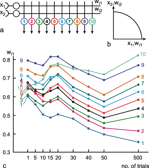
Fig. 13.2 Development of the mapping of an activation value onto a spatially distributed layer. (a) the net contains two input units and 10 topologically ordered output units, numbered from 1 to 10. (As the input vector is normalized to unit length, one scalar input, e. g., x1, would suffice). (b) shows the superposition of two coordinate systems, one for the (normalized) input vectors and the other for the weight vectors. As the weight vector are normalized, too, all vectors point to the unit circle. (c) Development of the weights wi1, i. e., the weights connecting the first input unit with the output units. Weight values are plotted along the ordinate. The weights are identified by the number of the corresponding output unit. At the beginning, the weights show a random order in the range between 0.6 and 0.8. During the training procedure, after 40 trials, the weight values are properly ordered, i. e., reflect the spatial position of the neuroids. After 500 trials, they cover the range between 0.3 and 0.9, showing an about equal distribution. The winner-take-all connections in the output layer, as well as the circuits for normalization and for learning are not shown
Feature maps are an interesting concept of how gradients could be trained that map the topology of the outside world. As mentioned earlier, the problems of normalization, which require a global knowledge, and the reduction of input space could be solved when applying the network shown in Figure 12.6 to competitive learning. After a neighbourhood is introduced in layer 3, this network can also be used to train feature maps.
In the sense described so far, feature maps can be considered capable of producing an internal representation of the sensory environment. In order to use this approach to control motor output, the system was extended by Martinez et al. (1990) and Ritter et al. (1992) in the following way. In the example presented here, a three-joint robot arm should move its end effector to a given target. The position of the target, corresponding to the desired position of the end effector in three-dimensional space, is given by two cameras that provide two coordinates each thus, taken together, a four-dimensional vector. Therefore, the desired position of the robot end effector can be represented by four input neuroids representing the x and y coordinates of the two camera frames. When only target positions on a horizontal table, i. e., in a two dimensional plane, are considered, a mapping from this four-dimensional input vector onto a two-dimensional layer of, in the example of Figure 13.3, 15 x 24 neuroids is possible using the procedure described above ( Ritter et al. 1989 ). In this mapping, the position of each of these 15 x 24 neuroids within the layer corresponds to a position on the table. The development of this map is illustrated in Figure 13.3a, b, c in a similar way as was shown in Figure 13.2c, but now for a two-dimensional situation. The two weights of each unit are projected on the table position such that each unit (to be more exact, its weight vector) is represented by a point on the table. To show how the topological arrangement of the units in the 15 x 24 layer fit the position on the table, the weight vectors of neighboring units are connected by lines. At the beginning, because of the randomly chosen weights, no order can be seen (Fig. 13.3 a). During learning (Fig.13.3 b, c), the initial random arrangement changes into a well-ordered map (b, 500 trials, c, 10000 trials). Thus, after learning, the 15 x 24 layer represents positions on the table for an arbitrary arrangement of the two cameras. Of course, a change of the position of a camera requires a new training session. However, small movements of the cameras need only minor changes of the weights, which means shorter learning sessions. Interestingly, when the central part of the workspace is more frequently used during the learning process, a non-uniform mapping results, showing a better spatial resolution in this central part (Fig. 13.3d).
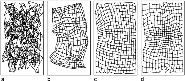
Fig. 13.3 Development of a two-dimensional feature map. Positions on a horizontal table are viewed by two cameras. Therefore, each point on the table produces a four-dimensional vector (two coordinate values for each camera frame). This vector is mapped on a two-dimensional grid consisting of 15 x 24 neuroids. The figure shows the values of two weights of each unit, corresponding to the input from one camera frame, projected onto the table. Two corresponding weights are shown by one point. Weight vectors of neighboring neuroids are connected by lines. The initial random distribution (a) becomes more ordered after 500 training procedures (b) and shows an about stable state after 10000 training sessions (c). When positions near the center of the table are presented more often, the mapping shows a higher spatial resolution in this central part (d) ( Ritter et al. 1989 )
In order to control the movement of the robot arm, Ritter, Martinez, and Schulten used a second mapping by which each unit of the 15 x 24 layer was associated to three output values corresponding to the positions of the three robot joints. Furthermore, Figure 13.3 is based on a more complicated example, which also includes the dynamic properties of the robot arm. Both of these extensions lead to the concept of local linear map networks (LLM nets) in which each neuroid is assigned a local linear mapping that describes the transformation in a local region of the input space (for further details, see Ritter et al. 1992 ).
When the competitive learning procedure is applied to a neuronal layer with a defined neighborhood, topological mappings can be learned. Feature maps can also be used to transform scalar input values into an excitation of spatial positions. The mapping can be distorted to reflect the frequency distribution of the input vectors.
Historical Note
An early sketch of a system which could be described as a distributed neuronal system was presented by Exner (1894) . It represents a "center for motion perception" (see Franceschini et al. 1989 ). Sequential flashing received by the receptors of the human retina creates an impression of movement and the eye is moved in the direction of the apparent movement. Exner proposed a wiring diagram to explain this finding (Fig. B7.1). The nodes marked by letters a - f represent receptors of the retina. An excitation of one receptor proceeds in all four directions. These excitations are summed up at the four centers E, S, Jt and Jf. These, in turn, excite the motor centers a1 - a4 which are connected to four eye muscles (Mus. int., Mus. sup., Mus. ext., Mus. inf.) moving the eye. The delay required to detect the movement (see Part I - Box 2 ) was assumed to be due to the finite conduction velocity of the excitation along the nerve fibers. Connections C are assumed to transmit the signals to the cortex.

Fig. B 7.1 Probably the first sketch of a neural network, as proposed by Exner (1894)
First detailed theoretical investigations of the properties of neural networks were performed by the independent development of a two-layer feedforward system which was called Perceptron by Rosenblatt (1958) and Learning Matrix by Steinbuch (1961) , and the investigations of spatial high-pass filters, namely lateral inhibition in the visual system ( Reichardt and Mac Ginitie 1962 , Varju 1962 , 1965 , Ratliff 1965 ).
Following the important, but partly misinterpreted book of Minsky and Papert (1969) , most investigators lost interest in this field. About twenty years later, two different approaches gave an extraordinary thrust to the investigation of massively parallel systems. One approach was given by the seminal papers of Hopfield ( 1982 , 1984 ) showing the interesting properties of recurrent networks. The other was the paper of Kohonen (1982) on the self organization of feature maps. The latter idea was to a large extent proposed 6 years earlier by Willshaw and von der Malsburg (1976) , but this paper apparently was before its time. At that time, there were no significant groups of scientists interested in this research. The third strong push came in 1986 by, again, two independent developments. Both LeCun (1985) and Rumelhart, Hinton, and Williams (1986) showed that the back propagation algorithm is capable to train feedforward networks having more than two layers. These papers removed the ban under which feedforward systems were put unintentionally by Minsky and Papert. However, even here a paper had already appeared about 10 years earlier ( Werbos 1974 ), and even in 1967 and 1968 Amari published results which, in principle, contain the necessary information, but neither were recognized as significant at the time.
Further important steps were the introduction of new training methods, in particular reinforcement learning ( Barto et al. 1981 ), competitive learning (for an early collection of papers see Amari and Arbib 1982 ), and genetic algorithms which have been introduced independently of the development of artificial neural networks ( Holland 1975 , Rechenberg 1973 ). Promising developments concern structured networks, i.e., networks consisting of specialized modules ("expert nets," Jacobs et al. 1991 ) and cascaded networks ( Fahlman and Lebiere 1990 , Littmann and Ritter 1993 ). The probably most important fields for future research concern the properties of asymmetric recurrent networks and the question of "active learning", where training examples are not presented to the network in random order, but where the net actively selects interesting training examples. Furthermore, the organization and self-organized development of large memories as well as internal models for action planning have to be considered.
As was mentioned earlier, recurrent networks represent the most general format of a network. However, there is yet no general theoretical framework that describes the properties of recurrent nets. Therefore, several networks will be discussed below which have a specifically defined structure. In the first example, most layers have only feedforward connections, and only one contains specified recurrent connections. This example is given by Elman (1990) (Fig. 14.1a). The system has an input layer, a hidden layer, and an output layer all of which are connected in a feedforward manner. The hidden layer, however, is not only connected to the output layer but also, in a simple 1 : 1 connection, to a further layer called the context layer. To form recurrent connections, the output of this context layer is also inputted to the hidden layer. Except for these 1 : 1 connections from hidden to context layer, the weights of which are fixed to 1, all other layers may be fully connected and all weights may be modifiable. The recurrent connections of the context layer provide the system with a short-term memory; the hidden units do not only observe the actual input but, via the context layer, also obtain information on their own state at the last time step. Since, at a given time step, hidden units have already been influenced by inputs at the earlier time steps, this recurrency comprises a memory which depends on earlier states (though their influence decays with time).
During operation, the input of the Elman net is provided with a temporal series of input vectors. To change the weights, the output can be compared with a desired output vector, and the generalized delta rule, for example, can be applied to change the weights. Thereby, the system learns to attribute an output not only directly to the actual input, but also to the temporal sequence of several subsequent input vectors.
As an example, Elman provided such a network with a random sequence of three words of different lengths, namely two, three, or four letters. The net was trained to predict the next letter in the sequence. Of course, a high error was observed when the first letter of a new word appeared. However, all following letters were predicted with low error. As the letters included also an end-of-word symbol, the word lenght was also predicted. In a similar experiment, a net was used consisting of 31 units in the input and output layers, and 150 units in the hidden as well as in the context layer. Small sentences consisting of two, three, or four words, selected from a set of 29 words, were given to the net. The complete input series consisted of a sequence of 10000 sentences (27 534 words). The net was trained to predict the subsequent word. After training, the state of the corresponding hidden layer was scrutinized in the following way. All hidden vectors for a given word were averaged, and, for each input word, these were then compared for similarity by means of a clustering technique. It turned out that different types of words appeared in separate clusters. For example, all verbs were grouped together, as were all nouns. The latter were again found in groups like animats and inanimats, the animats also containing different words describing humans as a subgroup. This means that the internal representation developed a sensible, implicit grouping of the words. This information is not explicitly given to the system, but is learnt only from the context in which the different words appear in the input stream. It should be mentioned that a similar grouping could be obtained using the feature map approach ( Ritter and Kohonen 1989 ).
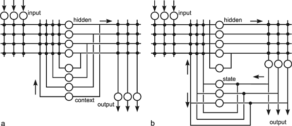
Fig. 14.1 Two networks with partial recurrent connections. (a) Elman net (b) Jordan net. Only the weights in the feedforward channels can be modified. The arrows show the direction of the information flow. These networks can be used to learn temporal sequences, i. e., to provide an output vector which depends on the temporal order of the input vectors. Conversely, for a given input vector, a series of output vectors can be produced
Recurrent networks are particularly interesting in relation to motor control. For this purpose, Jordan (1986) proposed a very similar net (Fig. 14.1b). A difference is that the recurrent connections start from the output, rather than the hidden layer. Furthermore, the layer corresponding to the context, here called state layer, comprises a recurrent net itself with 1:1 connections and fixed weights. Another difference is that the network was used by Jordan so that a constant input vector is given to the net, and the output of the net performs a temporal sequence of vectors. The variation in time is produced by the two types of recurrent connections, namely those from the output layer to the state layer and those within the state layer. For each input vector, another temporal sequence can be produced. However, as the Elman net and the Jordan net are quite similar, each can be used for both purposes. Both types of networks have the advantage that only weights in the forward connections are modifiable and therefore no special training methods for recurrent nets have to be introduced.
Examples of partially recurrent networks are described. Such networks can be used to learn temporal sequences such that they produce an output vector for a given sequence of input vectors, or, reversely, produce a series of output vectors for a given input vector.
When we are interested to construct a recurrent neural network that shows a complex, but given dynamic behavior, backpropagation through time can be applied as described above. A much simpler solution, however, is to use echo state networks ( Jaeger and Haas 2004 ). An echo state network consists of two parts, a recurrent network with fixed weights, called dynamic reservoir, and output units that are connected to the neuroids of the dynamic reservoir. Only one output unit is depicted in Figure 14.2 for simplicity. The dynamic reservoir consists of recurrently, usually sparsely connected units with logistic activation functions. The randomly selected strengths of the connections have to be small enough to avoid growing oscillations (this is guaranteed by using a weight matrix with the largest eigenvector smaller than 1). To test this property, the dynamic reservoir, after being excited by an impulse-like input to some of the units, may perform complex dynamics which however should decrease to zero with time. These dynamics are exploited by the output units. These output units are again randomly and recurrently connected to the units of the dynamic reservoir. Only those weights that determine the connections from the dynamic reservoir to the output units are learnt. All other weights are specified at the beginning and then held fixed.
To learn a given dynamic behavior, the output units receive this dynamic function via an external input that is only used during the training procedure: by this way the output units are “forced” to show the appropriate behavior. Via the recurrent connections to the dynamic reservoir the latter is excited to show any probably complex dynamic behavior. This is again read by the output units the weights of which now have to be changed in a way that they exactly produce the forced activity of the output units. Learning of the weights can simply by done by application of the delta rule to the output units. If learning is finished, the complete system, dynamic reservoir plus output units, has developed an attractor that produces the desired dynamics which are stabilized against small disturbances. The units of the dynamic reservoir can also be driven by external input such that different dynamics could be produced depending on this input signal. A quite similar approach, called “liquid state machines” has been proposed by Maass et al. (2002) , the main difference being that the latter is applied to spiking neurons.
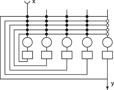
Fig. 14.2 Echo state network. The dynamic reservoir consists of recurrently connected units. The output units are recurrently connected to the units of the dynamic reservoir, but only the output connections (open circles) are due to learning. All the other weights (closed circles) are fixed before learning starts.
Echo state nets consist of a dynamic reservoir, a recurrent net with fixed weights. The output units can be interpreted as to exploit the different local dynamics of the dynamic reservoir and superimpose them to achieve the desired dynamics in a way that reminds of the composition of Fourier components.
With respect to their dynamical properties, recurrent neural networks may be described as showing fixed point attractors (e.g. Hopfield nets or MMC nets,
Chapter 14.4
), periodic attractors (e.g. Fig. 11.6), or chaotic attractors (Fig. 11.10). How is it possible to design a neural network with specific dynamics? Dynamical systems are often described by differential equations. In such cases the construction of a recurrent network is easily possible: Any system described by a linear differential equation of order n can be transformed into a recurrent neural network containing n units (Nauck et al., 2003). To this end, the differential equation has first to be transferred into a system of n coupled differential equations of the order one. This will be shown using the example of a damped oscillator, which is described by
 , i.e. a second order differential equation with ω being the squared angular frequency and r the friction. Introduction of the auxiliary variable
 gives the following two equations:


As explained in Part I – Chapter 8.10 and in Figs. 11.7 and 11.8, the easiest way to transfer such differential equations into a neural system is to integrate the equations which leads to


and in a discrete form to


These equations describe a two unit recurrent network with the weight matrix

The net is depicted in Figure 14.3. This is a recurrent neural network with nonsymmetrical weights showing damped (r ≠ 0 ) or undamped (r = 0) periodicity. Other examples of nonsymmetric recurrent nets are given in Chapter 11.5 showing properties of temporal low-pass filters or temporal high-pass filters. Such networks can easily be trained using the IC algorithm described in Chapter 12.4 (after Kühn et al 2006 ).
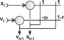
Fig. 14.3 A recurrent net showing damped oscillations. ω frequency, r friction
Any linear differential equation of order n can be transferred to a recurrent network containing n units which permits to construct networks of very different dynamics.
A specific type of recurrent neural networks that show fixed-point attractors and that are particularly suited to describe systems with redundant degrees of freedom are the so called MMC nets. The easiest way to construct such a net is to start with a simpler version. Given a linear equation with n variables

for example a1 x1 + a2 x2 + a3 x3 = 0. Solving this basis equation for each xi gives a set of n equations as shown for n = 3:


Each of these n equations represents the computation performed by one neuroid. So the complete network represents Multiple Solutions of the Basis Equation, and is therefore termed MSBE net. Different to Hopfield nets, the weights are in general asymmetric (apart from the special case that all parameters ai are identical, i.e. a1 = a2 = a3), but follow the rule wij = 1/wji. The diagonal weights, by which each unit excites itself, could be zero, as in the example, or any positive value di, if all weights of this equation are further normalized by multiplication with 1/(di+1). Positive diagonal weights influence the dynamics to adopt low-pass filter-like properties, because the earlier state of this unit is transferred to the actual state with the factor d/(d+1). As di can be arbitrarily be chosen (di ≥ 0), the weights may then not follow the rule wij = 1/wji anymore. Starting this net with any vector a, the net will stabilize at a vector fulfilling the basic equation. This means that the attractor points form a smooth, in this example two-dimensional, space. This is another difference to Hopfield nets which show discrete attractor points. Furthermore, there are no nonlinear characteristics necessary.
This network can be expanded to form an MMC net. MMC nets result from the combination of several MSBE nets (i.e. several basis equations) with shared units. Such MMC nets can be used to describe landmark navigation in insects and as a model describing place cells found in rodents ( Cruse 2002 ). However, the principle can also be used to represent the kinematics of a body with complex geometry ( Steinkühler and Cruse 1998 ). As a simple example, we will use a three-joint arm that moves in two-dimensional space, therefore having one extra degree of freedom (Fig. 14.4a).
The properties of this type of network can best be described by starting with a simple linear version (Fig. 14.4b). As we have a two-dimensional case, the complete net consists of two identical networks. The output values correspond to the Cartesian coordinates of the six vectors shown in Figure 14.4a, the x coordinates of the vectors given by the net shown with solid lines, the y coordinates by dashed lines. To obtain the weights, vector equations drawn from the geometrical arrangement shown in Figure 14.4a are used as basis equations. This means in this case there are several basis equations possible. For example, each three vectors forming a triangle can be used to provide a basis equation (e.g. L 1 + L 2 - D 1 = 0). As a given variable (e.g. L 1) occurs in different basis equations, there are several equations to determine this variable. The idea of the MMC net is to actually perform all these calculations in parallel, take the mean of each variable and use these mean values of each variable for the next iteration; therefore the name MMC: Mean of Multiple Computation, a principle exploiting the redundancy of the task.
When this network obtains as input the coordinates of vector R (which determines the position where the arm should point to), for example, after relaxation it describes a geometrically possible solution for the arm. In this way, the inverse kinematic problem ( Chapter 14.5 ) is solved.
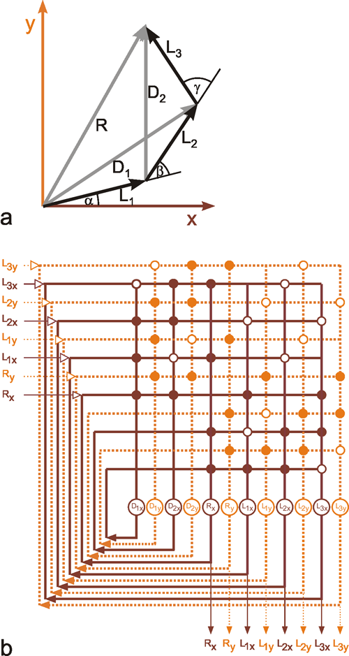
Fig. 14.4 (a) An arm consisting of three segments described by the vectors L1 L2, and L3 which are connected by three planar joints. The joint angles are α, β, and γ. The position of the endeffector is described by R. Furthermore, two additional vectors D1 and D2, describing the diagonals, are shown. (b) The linear version of the MMC net. The output values represent the components of the vectors R, L1, L2, and L3 (lower line). Solid lines represent the subnet for the x components, dashed lines that for the y components. To calculate the inverse kinematics, the components of R have to be provided as input for the net. However, any other combination of input values could be chosen instead. The possible input values are shown on the vertical column at the left. For the chosen input, the recurrent line is suppressed, and only the input value is fed into the net, symbolized by the small arrowheads
In this linear version, the lengths of the arm segments are not fixed, which corresponds to a robot with rotational and telescopic joints. To maintain constant segment lengths and thus constrain the arm to have only rotational joints, nonlinear elements have to be introduced. This is shown in Figure 14.5 where the joints angles are calculated using the coordinate values (P). The corresponding inverse calculation is performed by (Q). Furthermore, rotations of the local coordinate systems are necessary (T). In this version, the input and the output vectors consists of five components, two describing the position of the end effector in Cartesian coordinates (Rx, Ry), and three describing the joint angles (α, β, and γ). All geometrically possible arm configurations form a three-dimensional subspace of this five-dimensional vector space. Each point of this three-dimensional subspace can serve as an attractor to which the net can relax. This shows again that the attractor points form a smooth space, in contrast to Hopfield nets where the attractors comprise discrete points. Such a relaxation occurs for each arbitrarily chosen combination of three or less input components. This means that even if only one component is specified at the input, a five-dimensional vector appears at the output which, first, fulfils the input specification ("pattern completion") and, second, describes a geometrically possible arm configuration.
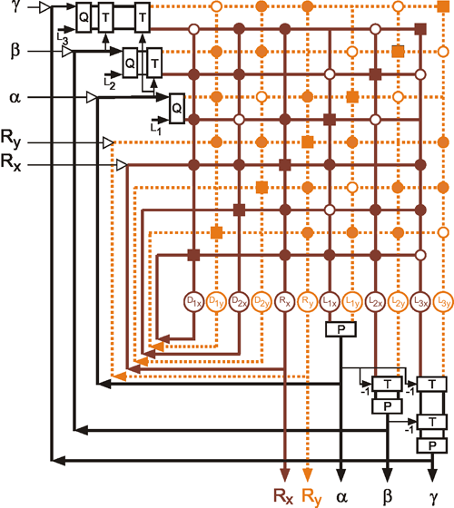
Fig. 14.5 The MMC net as shown in Fig. 14.4b, but with nonlinear subsystems in the feedback loops. In this case the input and output vectors contain the components Rx and Ry, describing the position of the endeffector, as well as the joint angles α, β, and γ. The nonlinear systems P, T, and Q are explained in the text.
Thus, we can, for example, solve the inverse kinematic problem by giving Rx and Ry as input values. Or, we can solve a mixed problem by, for example, specifying Rx and α. Both tasks are underdetermined and the system by itself finds a solution. The actual solution depends on the starting configuration of the arm. If Rx, α, and β are given at the input, the situation is determined and the net provides the remaining values Ry and γ. Thus, the inverse, the direct, and any mixed kinematic problem can be solved. Furthermore, any special constraints of the variables (e. g., joint limits) can be introduced. In this way, the MMC-type network can be used as an kinematic inverse model which allows for very different solutions of the redundancy problem and which can easily cope with limitations of the joint space or the workspace. The net can even solve the task when Rx and Ry values are given that describe a position outside the workspace of the arm. In this case, the arm tries to reach this position as far as possible and points in the direction of the position determined by Rx and Ry.
An MMC net is shown that relaxes to a stable state corresponding to a geometrically correct solution even when the input does not fully constrain the solution. The underlying idea is that several geometrical relationships are used to calculate the same value (e. g., angle α) several times in parallel. The final output is then obtained by calculation of the Mean value of these Multiple Computations (MMC). These mean values are then fed back for the next iteration. Applied to a body model, this MMC net serves as an internal model to provide the inverse kinematics. It can exploit the full range of geometrically possible arm configurations and permits the introduction of variable constraints. Representing a holistic model, there is no separation possible between a motor system and a sensory system. Furthermore, simpler versions are shown that are able to represent static or dynamic situations.
Using recurrent neural networks like Jordan nets or MMC nets for the control of behavior, i.e. use their output for direct control of the actuators, would mean that no online feedback was applied ( Part I –Chapter 8 , open loop control). However, feedback control is helpful in a nonpredictable world. A complication can occur in a feedback control system, (which was not addressed in Part I - Chapter 8 ) when the controlled variables and the desired variables are different in nature. This is the case, for example, when controlling the movement of a two- (or three-) joint arm in a plane. Let us assume that the tip of the arm has to be moved along a trajectory given in x, y (e. g., Cartesian) coordinates of the plane (Fig. 14.6); the motor output of the system has, however, to be given in joint angles. Therefore, in the feedback loop, the angle values of the joints have to be transformed to position values of the tip. This transformation (α → x) is called the direct kinematics (DK) and is solvable for an arbitrary number of joints. The x, y coordinates can then be compared with the desired coordinate values (Fig. 14.7a). The error signals given in Cartesian coordinates have to be transformed into angle values (joint coordinates). This transformation (x → α) is called the inverse kinematics (IK). It is solvable if the number of degrees of freedom in workspace and jointspace is the same (e. g., two coordinates x, y; two joints α, β), but there is no general solution for the so-called redundant case. This occurs when the jointspace has more degrees of freedom than the workspace (Fig. 14.6b). In this case, a given tip position could be reached by a number of different arm configurations (α, β, γ) and therefore no unique solution is possible. In this event additional constraints have to be introduced. Examples are minimization of energy consumption or of movement time.
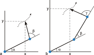
Fig. 14.6 A two-joint arm (a) and a three-joint arm (b) moving in a two dimensional (x-y) plane. When the tip of the arm has to follow a given trajectory (dotted arrow), in the redundant case (b) an infinite number of joint angle combinations can solve the problem for any given position of the tip
Several models are proposed to control the movement of such a redundant (or nonredundant) arm. One model corresponds to a schema shown in Figure 14.7a, where DK and IK may represent feedforward (e. g., three-layer) networks, computing the direct (DK) and inverse kinematics (IK) solutions, respectively. (In the redundant case, IK has to represent a particular solution). Depending on the sensory system applied, the DK system might belong to the process, for example when the position of the tip of the arm is registered visually, or it might be part of the neuronal system, for example if joint angles are monitored. In principle, the process can be controlled with this feedback network. However, since in biological systems information transfer is slow, this solution is not appropriate for fast movements because long delays can lead to unstable behavior ( Part I – Chapter 8 ). A further complication of the control task occurs if there is a process with nonnegligible dynamic properties ( Part I - Chapter 8 ). This means that computation is more complex because not only the kinematics but also the forward and inverse dynamics have to be determined. A simple solution of this problem would be to expand the system by introducing an internal (neuronal) model of the process (Fig. 14.7b, FM). By this, the behavior of the process can be predicted in advance, e. g., inertia effects could be compensated for before they occur. This prediction system is called forward model (FM). Usually, although depicted separately in Figure 14.7a, in this case the DK is considered part of the forward model. In other words, the FM predicts the next state of the arm (e.g. position, velocity) if the actual state and the motor command is known. Note that the network consists of serially connected IK and FM (including DK) forming a loop within the system and can therefore be represented by a recurrent neural network. The additional external feedback loop is omitted in Figure 14.7b, but is still necessary if external disturbances occur. It should be mentioned that the output of the FM, i.e. the predicted sensory feedback, could also be compared with the real sensory feedback. As described above ( Part I – Chapter 8.9 ), this could be used to distinguish sensors effects produced by own actions from those produced by external activities.
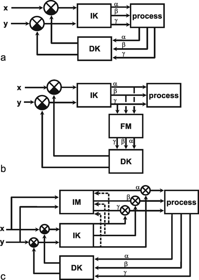
Fig. 14.7 Three ways of controlling the movement of a redundant (or non redundant) arm as shown in Fig. 14.6. DK, IK: networks solving the direct or inverse kinematics, respectively. FM: forward model of the process. IM: inverse model of the process. The dashed lines in (c) denote the error signals used to train the inverse model
An even faster way to solve this problem would be to introduce the inverse model (IM), which corresponds to the inverse kinematics, but may also incorporate the dynamic properties of the process (Fig. 14.7c, upper part). Given the desired new state of the arm, the inverse model does provide the necessary motor command (x -> α) to reach this state. Using such an inverse model, the process could be controlled without the need of an internal feedback loop.
How can we obtain a network for the inverse model? Kawato and Gomi (1992) discuss several possibilities and proposes the following circuit. Starting with the simple network shown in Figure 14.7a, a naive net to learn the IM is connected parallel to the IK net, as shown in Figure 14.7c. At the beginning of learning, the output of the IM is weighed with zero. Thus, due to the slow feedback controller, only slow movements can be performed. However, during the movements, the IM net can be trained by using the output of the IK module as error signals which can, for example, be backproped through the IM net, thereby improving its performance. Thus, with time, the output of IM could be attributed higher weights, and the IM module can exercise an increasing control over the process. (One measure to determine the relative strength of the IM influence might be something like the inverse of the averaged error). After learning, the feedback signals are no longer necessary for normal performance. However, if the properties of the system change, they are needed for new training.
This arrangement has the advantage that an IM net can also be found for a redundant system, i.e. a system with extra degrees of freedom (e.g. Fig. 14.2b) provided that the lK net is given. However, the IK net provides only one solution depending on its internal structure, i. e., the kind of constraints chosen, and only this solution can, of course, be learnt by the IM module.
Control of motor output can be improved by applying forward models and/or inverse models of the process. The former is used as predictor of the expected sensory feedback, the latter for the control of the process.
Most artificial networks considered usually code the signals in the form of varying excitation of the individual neuron. This “intensity coding” is an appropriate general solution for artificial neuroids because they have a very good resolution compared to biological neurons. In biological neurons the amount of transferable information is much smaller. Therefore, in biological systems intensity coding can only be used in a limited way and this limitation is compensated by application of even more extensive distributed architectures than are used in usual artificial neural networks. This can be done for example by application of range fractionation. In this case, neurons still use intensity coding, but via nonlinear characteristics each neuron covers only a limited section of the complete range to be transmitted. Another way is to apply spatial coding. Some examples will be explained below.
Spatial to spatial: The most obvious example of spatial coding is given in situations in which already the input information is represented in a spatial domain, as is the case for retinal images or for somatosensory input. In these cases we find spatial low pass filters and spatial high pass filters as described above (Chapt. 10.1 – 10.3).
Coarse coding: One might assume that a spatial coding system using discrete units may have the disadvantage of limited spatial resolution. This is indeed the case if the units are not connected and form strictly separated channels. If there is an overlap between neighboring units, one might assume that the spatial resolution is even worse. However, the opposite is the case. A spatial low pass filter, providing such an overlap, allows to transmit also intermediate values. These are coded in the form of excitation ratio of neighboring units. (see Chapt. 10.1). Therefore, “coarse coding” ( Rumelhart et al. 1986 , Baldi and Heiligenberg 1988 ) is a way to increase the spatial resolution beyond the discrete nature of neuronal arrangements. A special example is color vision: we have only three color units but can see a huge number of intermediate colors). If the weight function of this low pass filter is chosen appropriately, in principle a completely smooth information transfer is possible.
Temporal differences to spatial difference: Another example is given by the system which has to detect the direction of a sound source. The information is given (in part) by the temporal difference between the signals received by both ears. The neuronal system transfers this temporal difference into a spatial difference (Fig. 15.1), using a simple feedforward network and coincidence detectors (e.g. multipliers). The system exploits the fact that in neuronal systems information transmission is relatively slow. This circuit allows very high temporal resolution (e.g. 0.03 ms in humans).
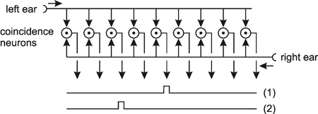
Fig. 15.1 Calculation of temporal difference using spatial coding. If the stimulus reaches right ear and the left ear at exactly the same time, the coincidence neurons will be excited that are positioned in the center of the chain (1). If the left ear, for example, is stimulated earlier, the position of the excited coincidence neurons will shift to the left side (2)
From intensity coding to spatial coding: A Kohonen network with a low number (e.g. one) of input channels and a high number (e.g. 10) of output channels can be considered as to transform an intensity coded signal into a topologically coded neural chain. This output unit code the information in the spatial domain (see Fig. 13.2). The distribution of the output signal could of course be sharpened by application of a subsequent WTA net.
Calculation of mean values: The coarse coding principle mentioned above can also be exploited in another way. Assume that several (e.g. n) values are represented, each by its neuronal chain, with one unit of the chain excited. The task is to determine a mean value of these n values. (for example when the same value has been measured by different sense organs). For simplicity of explanation assume further that the chains all consist of k units.
To calculate the mean of n values represented spatially on n neuronal chains with k units, each of these n chains (Fig. 15.2, Spatial Input 1 and 2) has to be connected to a new chain with k units (Fig. 15.2, Spatial Output). However, the connections are not 1:1 but represent a spatial low pass filter with a broad weighting function covering the whole range of the chain such that e.g. excitation of the leftmost input unit gives a non zero output to the rightmost unit of the next layer. The form of the weight function must not be linear but has to decrease with a steeper slope near the center and a slope getting continuously smaller to the sides. In this case the superposition of all weighted inputs gives a function the maximum of which corresponds to some kind of mean value (it rather corresponds to the mode vale than to the arithmetic mean). If this output function is given to a WTA net with k units, the maximum, i.e. the mean can be clearly detected. This net has a further advantage: Input values far away from the “center of gravity” do not contribute a lot, which means that this calculation is not very sensitive to outliers. In particular, this is true in the case when one value is not available at all, i.e. when all values of this chain have zero excitation. This means that no knowledge is necessary as to how many values are used to determine the mean value compared to a system using intensity coding where the sum has to be divided by n.
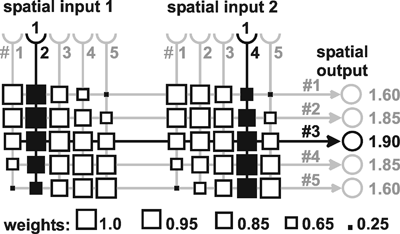
Fig. 15. 2 Calculating the mean value of two spatially encoded scalar. Output neuroids are drawn as open circles, input neuroids as semicircles. Arrows represent exciting connections, the weights are represented as squares. Two spatially encoded scalars "2" and "4" are given by an excitation of 1.0 of the respective neuroids (black pathways, input neuroid #2 and #4, respectively). In that case, the highest activation can be found in output neuroid #3. If necessary, the mean value can be computed by a winner-take-all network (not shown) at the right side (after Linder 2005 ).
Deviation, confidence measure: This network can also be used to determine a measure for the deviation between the different input values. The more compact the distribution of the original input values, the higher is the maximum obtained by this superposition. This means that the absolute value of the maximum excitation can also be used as a measure for the deviation of the input values from the mean. A good match between the input values gives a high maximum value. Therefore, the value of the maximum can be interpreted as a confidence measure for the mean value (see circular statistics). If in a subsequent calculation using this mean value is applied, the confidence measure could be used to weight the contribution of this mean value.
Multiplication: A simple solution to multiply spatially encoded input values with a constant factor is to arrange the connection matrix between input and output layer in a manner corresponding to the desired factor: for a factor of 0.5, every unit in the output layer is connected to two succeeding units in the input chain; for a factor of 2, only every second output unit gets connected to one of the input units. A proposal for multiplication of two variable inputs is given by Hartmann and Wehner (1995) .
Temporal signal is integrated and transformed to a spatial output signal: The limited working range of real neurons becomes particularly obvious when a signal has to be integrated (see e.g. path integration in ants). An elegant solution to cope with this problem is the Hartmann-Wehner integrator (Fig. B6.1). The distance moved by the animal is given by an intensity signal. The circuit integrates over this input ( i.e. calculates the sum) and therefore provides a signal which represents the actual position of the animal (= whole distance traveled). The spatial resolution of this system can be made arbitrarily good provided a high enough number of units is spent. The central units in Fig. B6.1 that represent the actual position comprise yes-or-no units a property which makes them relatively error tolerant. When this chain of neurons is closed to form a ring, this ring is an elegant solution to represent angular information, in the case of navigating ants the direction of walking.
(This system may be further improved when the units of the central chain could form a kind of distributed maximum (kind of softmax) instead of the strict yes-or-no behavior of the H-W integrator)
Summation: Summation can be seen as the computation of a mean value (see Calculation of mean values), followed by a multiplication with a constant factor, which corresponds to the number of input values considered for determination of the mean value. A network for summation can thus be assembled from previous cases (i.e., Calculation of mean values and Multiplication).
Another possibility for the summation of two values is given by a combination of two of the aforementioned Hartmann-Wehner integrators, say I1 and I2 (Fig. 15.3) as shown by Linder (2005) . They are connected in such a way that each unit of I2 which codes for a negative value is connected with the s- input neuron of I1 and the s+ input neuron of I2. Vice versa, each unit of I2 coding for a positive value is connected to the s+ input neuron of I1 and its own s- input neuron. Since the region at zero is not connected to any input neuron, the system stabilizes as soon as I2 represents a value of zero. At this time I1 contains the spatial representation of the sum of both values formerly represented in I1 and I2. This architecture can be nested for the summation of more than two values. In each case, the number of values to be summed has to be known in advance.
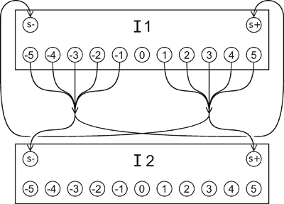
Fig. 15.3 Circuit for the summation of two spatially encoded values. Neurons are drawn as open circles, arrows represent exciting connections. Each box (I1 and I2) represents a Hartmann-Wehner Integrator (see Fig. B 6.1). The left and right shift neurons are displayed as s- and s+, respectively. Two values are initially represented in I1 and I2. After stabilization, the sum of both values is represented in I2. See text for an explanation (after Linder 2005 ).
Subtraction: While subtraction can be done similar to addition by a combination of integrators, there are two alternatives ( Linder 2005 ). In the examples described above, a neural chain is used to code a value in a way that only one unit of the chain is excites and the position of this unit within the chain represents the value. As one alternative, a complete set of neighboring units might be excited and the number of excited units represents the value. In this case, a subtraction of value a from a value b (i.e.: a - b) can be performed when all excited units representing the value b inhibit in a 1:1 connection the units of the chain representing the value a. The number of the units of chain b which survive this inhibition correspond to the value of (a – b).
Another alternative is obtained if activation is assumed to spread in each neuronal chain unilaterally: We employ two chains of neuroids situated next to each other. One codes for the x value, the other for the y value (Fig. 15.4). We assume the neuronal chains to represent exactly the same input space, such that for every neuroid the neighboring neuroid in the opposite chain codes for the same range of data. Let us assume that neuroid D (an intensity coded unit) receives the positive part of the difference x - y, and the corresponding neuroid D’ receives the negative part of the difference x - y. Furthermore, we assume each neuroid of one chain to inhibit (small filled circles in Fig. 15.4) all axonic branches of the neuroids in the other chain that are located towards one common direction (e.g., upwards in Fig. 15.4). Finally, we assume unidirectional exciting connections between directly neighboring units within each chain (Fig. 15.4, upward arrows).
What are the properties of this network? If directly opposing neuroids are activated in each chain (i.e., x = y), they reciprocally inhibit each others output and the upward spread of activation. Therefore, none of the output neuroids is excited. If, on the other hand, x ≠ y, both chains are activated at distinct locations (in the example of Fig. 15.4: unit 2 and 5'). While the activated neuroid on one side (left side in Fig. 15.4) can promote its activation in upward direction, the spread of excitation along the neuronal chain is inhibited on the other, in our example the right side. This spread of activation is continued until the activation reaches the neuron next to the single activated neuroid in the other chain (unit 5 in Fig. 15.4 ), which inhibits further spread of activation. Thus, on the left side, neuroids 2, 3, 4 and 5 are activated (as the spreading of activation takes time, the properties of this network in the time domain qualitatively correspond to that of a low pass filter). As neuroids 5 in both chains suppress each others output, only units 2, 3 and 4 promote their activation to the output. The activation of neuroid D (3) is therefore proportional to the difference between x (unit #5) and y (unit #2). The output unit D’ does not receive any input in this case. Since the architecture is symmetric, the outcome is reversed for reverse input constellations: if x < y, the activation of the output unit D’ is proportional to the difference, while D remains inactive. This architecture therefore performs the subtraction of spatially encoded values.
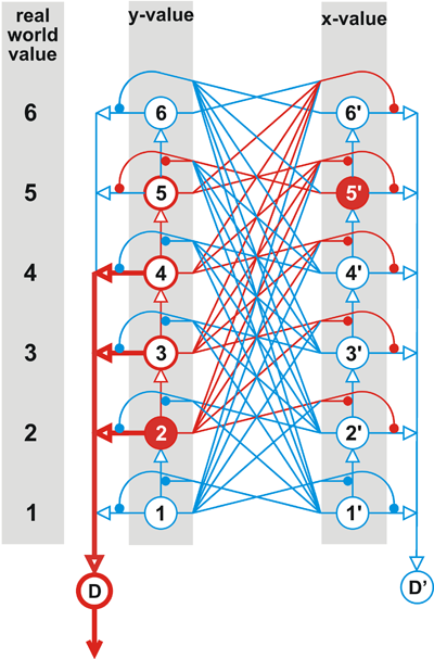
Fig. 15.4 A neural network for the subtraction of two spatially encoded values x - y. Neuroids are drawn as big circles, lines ending in little filled circles represent inhibiting connections. Exciting connections are drawn as arrows. Each unit represents an angular value as indicated on the left. On both sides, the position of the filled neuron represents the y value to be subtracted. Arrows indicate exciting synapses, circles inhibitory synapses. D and D' represent intensity coded output units, each receiving input from every neuroid in its chain. If one neuroid coding for the y value is excited (#2), activation is spread upward to the position opposite to the activated neuroid of the other chain (#5'). Excited elements are shown by red lines. Activation of output unit D is proportional to the absolute value of the difference between x value and y value (and activation of D' for the absolute value of the difference between y value and x value, respectively)(after Linder 2005 ).
In a biological neural network spatial coding allows better resolution compared to intensity coding, but requires more neurons. Ways are explained as to how specific calculations can be performed using spatially encoded networks
As mentioned earlier, single neuroids or groups of neuroids may be considered as controlling separate behavioral units. These systems may be called "agents." Via the combination of such subsystems, models can be constructed which are capable of simulating the cooperation of different behavioral units and thus are the origin of more complex behaviors. This is of special interest when we study (and simulate), not a single type of behavior, but the question of how the different modes of behavior an animal is capable of performing are stored in the central nervous system, and how one of these is selected and recalled ("action selection"). In the field of "Artificial Life," such systems are used to control the behavior of "autonomous" robots which have become called animats ( Wilson 1987 ).
The classical view of how an "intelligent" system might be constructed could be described roughly as follows (Fig. 16.1): First, information from the environment is received by sensors. These data are then fed into an internal model. With the aid of this model and the goals inherent in the system, a decision is made in a planning unit as to which behavior will be executed. Following this, the corresponding behavior agent is selected which, in turn, executes the behavior via the effectors (shared by different behavior agents). In addition to this particular approach, which involves a central planning unit and follows the ideas of traditional Artificial Intelligence and earlier ethologists, other concepts are also discussed.

Fig. 16.1 Schematic presentation showing how in an animal or an artifical system the sensory input may cause a behavior action
A very simplified assumption is that single modes of behavior are realized in the form of input-output systems (agents) arranged in parallel, whose outputs run via a winner-take-all net. This net ensures that only one mode of behavior is executed, even though several behavior agents may have been activated by stimuli or internal motivation. According to this simplified view, the central nervous system would represent an accumulation of many stimulus-response (S-R) chains. Such a S-R chain is often regarded as a simple system. It should be noted, however, that this is not necessarily the case for a biological system. The identification and isolation of a stimulus signal against a noisy background may pose a formidable problem. Moreover, apart from a few extreme cases, the action following a stimulus requires a behavior sensibly adapted to the specific situation. For instance, grasping an object in itself presupposes a control mechanism of such complexity that so far, the problem has not been solved satisfactorily even for robots. Accordingly, when we speak here of a "simple" S-R chain, this may actually involve a highly complex system.
The parallel, equally weighted arrangement of individual behavior agents is contrasted with the observation that some modes of behavior seem to be "more equal" than others, suggesting that there may be hierarchies. A hidden hierarchical structure might be built into such a system by the way that the various agents arranged in parallel are endowed with different weights; therefore, they enter the decision-making winner-take-all net with varying degrees of intensity. The occurrence of displacement behavior, for example, can be simulated with the aid of a feedforward winner-take-all net (Fig. 16.2). Assume that two neuroids (e. g., "fighting," "fleeing") inhibit each other with equal intensity, both inhibiting a third neuroid ("sleeping") only slightly, and assume further that the neuroids "sleeping" is endowed with a constant excitation ("bias"). Normally, the most excited behavior wins (Fig. 16.2b, c). If fighting and fleeing are both excited equally, the neuroid "sleeping"- despite its own weak stimulation - may be the beneficiary when "fighting" and "fleeing" exhibit the same level of stimulation (Fig. 16.2d). The result becomes even more obvious if this system is followed by a second winner-take-all net.
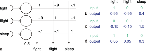
Fig. 16.2 A winner-take-all all net with unequal inhibitory influences. (a) The net has to decide which of three behavior agents (inputs fight, flight, and sleep) finally controls the activity, i. e., the output. The sleep agent is assumed to obtain a constant bias of 0.5. If only the fight agent (b), the flight agent (not shown) or only the sleep agent (c) is activated, the output corresponds to the input situation. (d) If fight and flight are equally active, the sleep agent will win. This simulates the occurrence of displacement behavior
The "subsumption architecture" proposed by Brooks (1986) , is endowed with both a hierarchical and a parallel structure. The individual agents (Fig. 16.3a) are arranged in parallel, as in the model described above. This means each agent is supported by its sensory apparatus, which initiates corresponding activations. However, the decision which of the different possible behaviors is to be executed is not determined via a winner-take-all net. Rather, there exists a hierarchically layered structure. A behavior agent arranged above can, in a state of activation, suppress the agent arranged below it, i. e., it can prevent the behavior controlled by the latter from being executed, and instead execute its own mode of behavior.
In Figure 16.3, this type of connection is shown by a circle containing the letter S. A simple example is shown in Figure 16.3b, which describes the control of a walking leg in, say, a six-legged machine. This leg is provided with two joints, the alpha joint for forward and rearward movement and the beta joint for lifting the leg up and down. During walking the "leg-down" agent is continuously excited and influences the "beta position" agent to adopt a value corresponding to a leg-down position (here assumed to be zero). Eventually the "leg-up trigger" agent receives a signal from a central timer, which is effective when the beta position signal is zero. The trigger signal elicits a positive valued output, which holds for a given time period ("clock"). This signal suppresses the signal from the "leg-down" agent. (Suppression in this special case corresponds to simple summation). The output of the "beta position" agent drives the motor of the beta joint and excites the "alpha protraction" agent. This suppresses the signal from the continuously excited "alpha retraction" agent to increase the value of the "alpha position" agent in order to move the leg in a forward direction. To obtain an increasing position signal, an integrator is used in the alpha position agent. If the alpha protraction agent provides a zero valued output, the alpha retraction agent moves the position signal to lower values. Figure 16.3b shows the arrangement of the agents (which Brooks has described as "augmented finite state machines") in a simplified version.
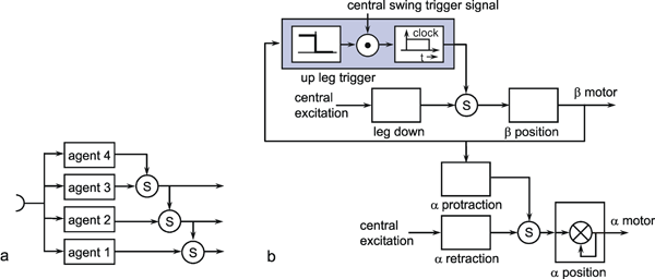
Fig. 16.3 (a) Schematic illustration of Brook's subsumption architecture. The different agents are arranged in parallel, but determine the actual behavior in a hierarchical manner. A superior agent, if active, may suppress (S) the output of the inferior agent and take over the control of the behavior. (b) A specific application of this principle for the control of the movement of a walking leg. The β motor output lifts the leg up or down, the α motor output moves the leg forward (protraction) of rearward (retraction). A central signal to trigger swing comes from a higher center which controls the coordination of the different legs. The swing movement continues for a prespecified time determined by a clock. During walking a continuous central signal excites the leg down agent and the α retraction agent. The α position agent contains an integrator, implemented here using a recurrent positive feedback circuit (after Brooks 1986 )
This subsumption structure has an advantage, among others, that if individual agents were to fail, the system may still survive. Another interesting aspect is that an "evolutionary" development of such a system is easily conceivable. A new agent could be introduced without reconstruction of the existing agents. The disadvantage is that this type of influence affecting individual levels has to be planned in great detail and is highly dependent on the internal structure of the levels as well as on the necessary interconnections between the behavioral modes.
The models considered so far are greatly simplified in that modes of behavior have been assumed to depend exclusively on stimuli ("sensory-, or data-driven models"). It has been known for a long time, though, that the response of an animal to a specific stimulus may also depend on its internal state, known as motivation, in relation to a specific mode of behavior. We will not go into detail concerning the existing, and greatly varying, definitions of this concept, but mention only two simple versions. Motivation can be equated with the measure of intensity of a response to a specific stimulus. It may also be conceived of as an internal excitation that like an external stimulation, can influence the activation of a behavior agent. (See, e.g., bias influence in Figure 16.2). In the first case, the two quantities would be multiplied, and in the second, added together. By introducing a threshold for the initiation of the behavior, the difference between the two types of influence is blurred.
One example of the classic view is that of Lorenz' (1950) hydraulic model (Fig. 16.4a). The level of the water corresponds to the intensity of motivation, the weight to the intensity of the stimulus. The higher the motivation and the stronger the stimulus, the more intensive becomes the execution of behavior (the stronger the outflow of water). This corresponds to a multiplicative connection. Figure 16.4b shows a translation of this model into a circuit diagram (Hassenstein; in Eibl-Eibesfeldt 1980 ). If motivation is sufficiently high, though, a behavior can be initiated without a stimulus (vacuum activity). This corresponds to an additive connection. This is not shown in Figure 16.4 (But see Figure 16.5).
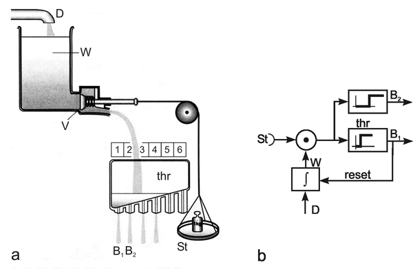
Fig. 16.4 The „psychohydraulic" model of Lorenz illustrating the possible cooperation of stimulus (weight, St) and motivation (height of the water level, W) to elicit a behavioral response (B) by opening the valve (V). Different behaviors may be elicited by reaching different threshold values (thr). The classical model further assumes a constant internal “drive" (D) to increase the motivation. Execution of the behavior diminishes the motivation level. (b) shows a simple circuit diagram with similar properties (after Lorenz 1950 ; Hassenstein, in Eibl-Eibesfeldt 1980 )
An open question is how the intensity of motivation can be influenced. In the simplest case, it would always be constant. But it could also depend on internal states, e. g., on a circadian clock or on a physiological state, such as the motivation "hunger" on blood sugar level. The latter case also suggests that it may be influenced by the error signal of a feedback system.
Moreover, as assumed in the specific case of the Lorenz model, the intensity of motivation could also increase with the time that has elapsed since the behavior was last executed. It could decrease, again as assumed in the Lorenz model, once the behavior has been initiated (or even when only particular sense organs, such as taste papillae, have been stimulated).
Before we go on to discuss models which combine "motivated behavior agents," a further principle of cooperation between different modes of behavior needs to be mentioned. Quite frequently, modes of behavior occur successively in temporal terms. These behavior chains cannot be described by a pure feedforward structure. A behavior chain, however, might simply develop because a behavior generates a situation in the environment which serves as an appropriate stimulus for a second behavior. Another possibility would be to assume that the individual agents are linked internally in such a way that, after completion of a behavior, the next agent is activated (see Figure 11.6). Between these two solutions there exists the possibility that by activation of one agent the threshold for the activating signal of the second behavioral agent is lowered, or the intensity of its motivation raised.
A combination of these possibilities is represented by the model of Maes (1991) . This has a simple structure but some very impressive features and will be shown here in a somewhat simplified version. The model assumes that the individual behavior agents that are arranged in parallel are linked with each other on two levels. Before discussing this in detail, we will deal with the structure of an individual agent. The intensities of stimulus and motivations are linked additively. The sum is called internal behavior activation. If this is greater than a given threshold, the signal reaches a winner-take-all net which ensures that only one mode of behavior is executed (Fig. 16.5a). This is the lower level connection between the agents. The model incorporates ten agents whose concomitant behavioral response is given in Figure 16.5b. Agents 1 -7 denote consummatory behaviors, agents, A, B, C appetitive behaviors. The latter three have no motivation of their own, i. e., they respond exclusively to sensory input. The intensity of motivation is assumed to be constant for some agents (e. g., fear, readiness to fight). For other agents, motivation diminishes once a behavior is actually executed (dashed line in Figure 16.5a). In proportion to the intensity of the internal behavior activation of an agent, the internal activations of other behavior agents can be raised or lowered. This is the upper level of cooperation. For this reason, linkages do not apply to all agents in the same way. Rather, the type of such a linkage depends on the type of agents, leading to the introduction of a hidden hierarchy. This is shown in Figure 16.5b. The rectangles represent the agents and the output corresponds to the internal behavior activations of the agent. Some of them inhibit each other. For example, a higher internal activation of fighting behavior inhibits the internal activation of flight behavior. Some agents increase the internal activation of another agent. These linkages are organized in such a way that they are capable of supporting temporal relations between two agents. For instance, if a specific behavior, such as "searching for food," is performed with greater intensity, the internal activation of the typically successive behavior, in this case feeding ("eat"), is also increased via a "successor" link (see solid arrows in Fig. 16.5b). At the same time, this raises the probability that, after the finding of food, the agent "eat" prevails over the other agents in the winner-take-all net and its behavior is executed next. High internal activation, but in the absence of an activating stimulus, which indicates high motivation, activates the typical preceding behavior via "predecessor" links. The high internal activation of feeding thus activates the agent "go to food," so that this behavior, which is appropriate in the circumstances, has a greater chance of being performed. In Figure 16.5 b, these linkages are represented by dashed arrows. Unless stimulated, internal activation decreases with a given time constant. In this way, this agent is provided with low-pass properties, with the advantage that it does not respond to the high-frequency parts of the input signal as, for example, given by noise.
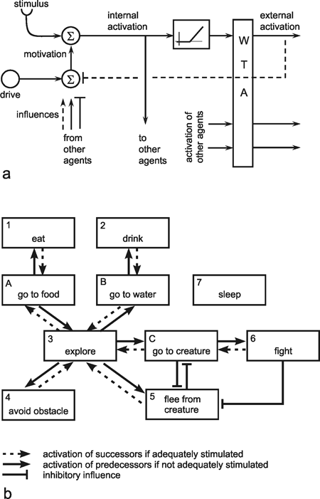
Fig. 16.5 (a) A behavior agent as used in the model of Maes. The excitation produced by stimulus and motivation are added to form the „internal activation". If above threshold, this competes in a winner-take-all net (WTA) with the internal activations of other agents. If it succeeds, the external activation of this agent elicits the behavior and inhibits the motivation. The motivation may also be influenced by an internal constant or varying drive (see Fig. 16.4) and by the internal activations of other agents. (b) The interior connections between the ten behavior agents used (the winner-take-all net is not shown). Solid arrows indicate an excitatory influence when the agent sending the information receives an adequate stimulus. These arrows point to agents which usually follow the behavior of the sender (e. g., eat follows go-to-food). Broken arrows point to another agent if the sender does not obtain an adequate stimulus. These arrows influence agents that are usually active before the sender is active (e. g. go-to-food is followed by eat) (after Maes 1991 )
Though simple, the model contains a number of interesting analogies to the behavior of real animals. The behavior of the total system depends both on the internal state, the motivations, and the state of the exterior world. Depending on the internal state, it is thus capable of responding in different ways to the same stimulus situation. It can respond "opportunistically," displaying drinking behavior when water happens to be available, although hunger may actually be greater than thirst. A system driven purely by motivations ("goal driven") would just search for food in such conditions. The system may also show displacement behavior. When readiness to fight and fear are both high and are suppressed by mutual inhibition, a third behavior may win the decision of the winner-take-all net as described earlier (Fig. 16.2). Like animals, the system is endowed with the phenomenon of varying attention. This means that, if a strong motivation exists for one mode of behavior, other equally important modes of behavior may be suppressed. It is thus possible that, in case of very great hunger, the model might not allow the behavior "obstacle avoidance" to become operational, and that it runs up against the obstacle. Due to the stimulation influences of the successive behavior, the system is endowed with the advantageous property of anticipation. The running toward a conspecific individual already raises the readiness to fight, even before the activating stimulus is registered. Lorenz's view that motivation increases continuously, if not for all, then at least for some modes of behavior, could be simulated by the introduction of an integrator into the motivation channel (as used in Figure 16.4b). This would mean that the system is also capable of displaying a vacuum activity. It should also be mentioned that, rather than influencing just one mode of behavior as described here, a given motivation might possibly influence several modes of behavior.
The problem with this "behavior-based" approach is that a considerable amount of intelligence is still necessary to design such a system. The question remains how animals solved this problem during evolution. How is it possible that a system can develop such structures without a specific designer? Tentative approaches have been made, for example, by Pfeifer and Verschure (1992) and Pfeifer (1995) . With the aid of Hebb synapses, a certain flexibility can be achieved by formation of new linkages of stimulus inputs and responses in the sense of classical conditioning (Pavlovian conditioning). In this case, too, some structure has to be prespecified though. In the example mentioned, a small, wheeled robot was constructed which has two built-in, i. e., hardwired, reflexes (Fig. 16.6a). When a collision detector has registered an obstacle, the robot drives rearward for a short period and then turns. Two collision detectors are mounted such that one detects obstacles on the right side of the body, leading to a left turn, whereas the other detector mounted symmetrically on the other side, elicits a right turn. Furthermore, a target detector is stimulated by a certain target signal, for example, a light source. The built-in reflex elicits a turn to the direction of the target, if the sensors are stimulated accordingly. In this case, the whole 360° range is observed by four sensors. If none of these detectors is stimulated, the robot moves straight ahead. These reflexes can be implemented using simple feedforward networks which, for convenience, are not shown in detail in Figure 16.6, but are represented by the bold arrows which connect both the c-layer (consisting of two units, "avoid") and the t-layer (consisting of four units, "approach") with the m-layer. In case of a conflict between the two reflexes, "collision avoidance" and "target approach," an unidirectional inhibitory connection influence operates to suppress the latter. With this net, the robot can move in an obstacle-cluttered environment and, if a target is presented, find the target by trial and error.
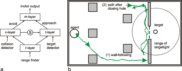
Fig. 16.6 (a) The structure of a robot to learn a new reflex. Two reflexes are built into the system: a connection between the collision detector and the motor output, producing an avoidance reflex, and a connection between target detector and motor output, producing a reaction to approach the target. In the case of a conflict the former reflex suppresses the latter (S). The connection between a third group of sensors, the range finder, and the other reflexes are learnt "automatically" using Hebbian learning. (b) shows some examples of how the robot behaves. It shows wall following (trace 1). Usually the robot finds the target after it has reached the range of target light source. If, in another experiment (trace 2), the hole in front of the target is closed, the robot "searches" in front of the closed door. As the collision avoidance net is stimulated quite often, the suppression of the approach net may become inhibited and the robot may move outside the range of the target light source (after Pfeifer and Verschure 1992 , Pfeifer 1995 )
Now a third, more complicated sensor is introduced. The sensor measures the distance of obstacles in a given angular range in front of the robot. The range sensor consists of a number of individual units (about 26, r-layer) each being responsible for a small angle range (3 degrees), covering a total range of about ± 40° around the forward direction. The output of these sensory units is now connected to all neuroids of the avoidance (c-layer) and approach subnets (t-layer).
The weights of these connections are zero at the beginning, but are changed according to Hebb's rule during the activity of the robot. Thus, when a collision detector is on, those units of the range sensor that are also stimulated will obtain stronger weights. Therefore, the weights develop such that, after learning, the range sensor signals achieve connections to the motor system which elicit similar behavior in similar situations as does the collision reflex. The same holds for the target approach reflex. Because the range sensor can detect objects from a greater distance than the collision detector, the number of collision decrease to zero during learning, and the robot shows much smoother trajectories.
In this way, different stimuli, which might occur at about the same time, can be learnt to replace each other, as is the case in classical conditioning. This is particularly interesting if, as in our example, the prewired reflex is a very simple one, and the more complicated connections have not to be hand-coded but are learnt automatically. Even better, it is learnt by using the perspective of the robot, and not that of an external designer, thereby taking the "situatedness" of the robot into account. The robot acquires its own knowledge, as it interacts with the environment. Because Hebb's rule is expanded by a decay term (see Chapter 12 ), the learning mode does not need to be switched off by an outside controller. Rather, the robot learns continuously.
The robot has developed a "wall following" behavior. (See trace 1 in Figure 16.6b). This continues even if the target is removed. An interesting behavior can be observed in another experiment. If the hole in the wall is closed, the robot moves along a trajectory similar to that shown in Figure 16.6b. If one describes the behavior of the robot as a psychologist would when observing a human subject, one might say the following: the animat follows the wall (trace 2 in Figure 16.6b) because it "expects" to find a target; it "knows" that the target is behind the wall, therefore, after "searching" along the wall for a given period or distance, it turns and tries again. However, the robot is not caught in this cycle. Rather, after some trials it "gives up," it "resigns." On the network level, the occurrence of this behavior can be explained in the following way: the "approach net" (Fig. 16.6a) is often inhibited. As the inhibitory connection has the property of a temporal low-pass filter, its output increases more and more, eventually inhibiting the approach net so strongly that the avoidance net completely governs the motor output for a prolonged time.
Of course, no "emotion units" for "expectation" or "resignation," or even special components for wall following are built into the system. The "psychological" interpretations are interesting, however, insofar as they show that, even if we have the strong impression of the existence of psychic states, they may not exist explicitly in the system in the form of special mechanisms. They might be just in the eye of the observer. This could even be the case for so-called higher systems. This question will be considered in Chapter 18 .
The construction of animats or autonomous robots is a significant tool to understand and test hypotheses concerning the control of various types of behavior. Different architectures have been proposed. An important step beyond purely sensory driven systems is the introduction of such central aspects as motivation. Another important, but so far generally unsolved, problem concerns the question of how systems can by themselves develop new sensible behavior.
Although systems as outlined in the last chapter could serve to describe many phenomena found in animal behavior, the question remains whether all known modes of animal behavior are attributable to systems based on relatively simple rules, or whether other structures are required for higher, so-called intelligent processes, i. e., modes of behavior that do not rely on given rules, but on reflecting, or reasoning. This question will be approached by considering a hypothetical series of animats that show an increasing number of abilities making these animats more and more similar to those highly developed systems that we believe to be intelligent. This hypothetical series, shown below, will briefly repeat several examples described earlier. To some extent, this series might reflect the evolution of the capabilities of animal brains.
The most simple types of animats contain a simple feedforward net consisting of two or three layers (an associative memory such as shown in Figure 10.9a) representing a system with direct sensorimotor coupling. The system can react to a number of different stimuli with adequate responses. The "choice" between the different behavioral responses is completely sensory-driven or "reactive." As described above, such a system already shows the properties of generalization and fault tolerance. Coarse coding (see Chapter 10.1 ) is already an inherent property of discretely structured neuronal systems.
Such an animat could be improved on the sensory as well as on the motor side. Examples of special developments on the part of the input (sensory) layer could be the introduction of spatial high-pass filtering (lateral inhibition) to make the system independent of absolute stimulus intensity. Special systems may be introduced to allow for dimension reduction to simplify the multidimensional sensory input (see feature maps, Chapter 13 ). An often used principle in the animal kingdom, which is therefore also adopted by animat constructors, is to exploit the physical properties of the environment to obtain relevant information in a simple way. Examples are arrangement of polarization detectors in the ant eye that reflect the average arrangement of the celestial map, allowing the animal to detect the position of the sun with sufficient accuracy even when only a small spot of blue sky is visible ( Wehner 1987 ). An exact mathematical solution for this problem is quite complicated. In motor systems potential energy can be stored during jumping by exploitation of the elasticity of muscles and tendons.
A further problem concerns phenomena of invariance. The size of a visual object on the retina, for example, depends highly on distance. Nevertheless, humans and many, though not all, animals treat such different appearances as the same object. Simple solutions providing size invariance in humans have been proposed by v. Holst (1957) . The convergence angle between the two eyes and the degree of accommodation of the lenses are used by the brain to calculate the absolute size of an observed object. An invariance phenomenon can also be observed in color vision. Subjectively, we have the impression of the color of a given object being the same even when the actually reflected color changes dramatically, depending on varying influences from the environment.
Another problem on the sensory side is that of feature linking. Different aspects of a given perceptual unit (size and color of an object for example) may be recorded in different parts of the brain. In other words, different subsystems can exploit the same input in different ways. (See also the well-known ambiguous figures). The question is how the different aspects are combined in order to be exploited by further layers which control the actuators. Hypotheses of how this question might be solved have been put forward by Eckhorn, Singer, and von der Malsburg (e. g., Eckhorn et al. 1988 , Engel et a1.1992 , von der Malsburg and Buhmann 1992 ), but will not be discussed here in detail. This problem also involves the question of how information storage is organized in a neuronal system consisting of many modules, which will be considered below.
Further improvements discussed in the following require the existence of recurrent connections within the system. (Possibly, these are already necessary to solve the questions of feature linking mentioned above). It is clear that a strict separation between motor and sensory sides is no longer possible when recurrent connections are introduced. One may rather distinguish between "low-level" feedback belonging to the motor side and "high-level" feedback corresponding more to the sensory side. Simple improvements on the motor side imply the introduction of control systems with negative feedback ( Part I – Chapter 8 ). Feedback can be used on several levels. Except for the classic form of continuous feedback, we find systems using intermittent feedback, i. e., the sensory signal is only used during defined time windows. Sensory input resulting from an action can, of course, also be used to trigger a new action (advance use), and thus as reference signal ( Cruse, Dean, Heuer, Schmidt 1990 ). Whereas the sense of a simple feedback system is to maintain the output value near a desired value, the circuit of the reafference principle ( Part I – Chapter 8.9 ) compares the input signal with a centrally produced "expected" value, ascertaining in this way whether a visually detected movement corresponds to that produced by its own motor system, thus, the reafference principle reflects some kind of "self-sense". Thereby the occurrence of external movements or a failure in the motor system could be detected.
An important capability of animats, and a necessity for evolved animals, is to cope with the problem of redundancy. This is due to both the sensory and the motor side. On the sensory side, most complex signals, e. g., in vision, can be interpreted in different ways, as mentioned below (e. g., figure-ground separation, ambiguous figures). On the motor side, a given goal can usually be achieved in different ways. On the lowest level, for instance, a observed object can be grasped by a manipulator, using the available actuators in different ways. For example, a human arm has more degrees of freedom than are necessary for most such tasks. This redundancy is even higher when the possibility of body locomotion is included. How does the system select between different possible behaviors, e. g., trajectories, and between different possible actuators, including their temporal order of activation? Simple solutions are known which imply fixed, preselected motor programs for given tasks, or fixed principles so as to minimize a given cost function (i. e., to find an energy optimal or time optimal solution). Recurrent networks are appropriate finding a unique solution from many possible ones when several limiting conditions have to be fulfilled. Therefore, recurrent nets may be used for this purpose ( Chapter 11.3 ).
We have so far only considered systems which are purely sensory-driven. An important property probably of most animals is to contribute actively to the control of their behavior. A simple example is a central oscillator, as described in Chapter 11.5 . Such central oscillators can be used to stabilize a behavior, making it independent of sensory influences, or as a kind of predictor system. The circadian clock of an animal, for example, is used to change internal parameters of the organism (e.g., body temperature) even before the external stimulus (e.g., light) occurs. More generally, animals and animats contain central pattern generators (CPG) that produce a special behavior (walking, flying). Simple examples are fixed action patterns where the activity of the CPG is only triggered by a sensory signal, but a CPG may also exploit sensory information during its activity. A simple example is given in Figure 11.9. In this case, the system consists of two fixed action patterns, the downstroke system and the upstroke system, but an oscillating system emerges when the environment is included as part of the system. A CPG may also use positive feedback, for instance to keep a behavioral state acting. Such central pattern generators may be used to control the input pattern in the sense of an active perception (see Box 8 ). By means of a central system only selected signals are further exploited by the system. The selection depends on the actual internal state of the system. This can already be observed in simple cases of "program dependent reflexes" where a stimulus is responded to in different ways depending on the internal state of the CPG. An example of this is the intermittent feedback mentioned above.
New problems arise when not one, but several CPGs are implemented in one system. These problems concern (a) structural arrangement and (b) how to select between these CPGs. On the structural side, one extreme case one could think of is a fully connected recurrent network, with the different functional units being more or less evenly distributed over the whole system, i. e., where all (or most of the) elements of the weight matrix show nonzero entries. Alternatively, one could think of separate subnets that may contain intensive recurrent connections within the subnet, but with only a small number of connections between different subnets. These subnets could be called modules, agents ( Minsky 1985 ), or schemata ( Arbib 1995 ). Because any number of intermodule connections could exist, it is not always possible clearly to define the modules. Apart from this problem, it should be noted that these modules might not only be arranged in parallel but also in some hierarchical order, and a module might therefore be regarded as consisting of several submodules.
Is there any advantage in modularity? If a system consists of subnets separated to some extent, the whole system is, intellectually speaking, easier to understand because these modules usually form smaller, and therefore more comprehensible, units. It may, then, be easier for an engineer, an animat and, for similar reasons, also evolution, to construct an animal from such modules. For example, if a new module is to be added to an already existing system, this is simpler if the modules are relatively separate. The old modules could be used nearly unchanged. For a completely interconnected system, however, most of the weights would have to be changed, if a new module is to be implemented (see expert nets, Chapter 12.6 ). On the other hand, modularity also has its problems. Apart from the problem already mentioned of how to select that module that will control the appropriate behavior, there are also structural problems. In the simplest case, these modules may be all arranged in parallel. Some hierarchy may be introduced according to the subsumption architecture ( Chapter 16 ). Other, more implicit hierarchical structures can be used as indicated in the approach of Maes ( Chapter 16 ). More explicit hierarchical arrangements may also be necessary. For example, one group of modules might form one CPG active in one situation, e. g., foraging, and another might exist for homing. Both groups, however, contain common submodules, e. g., to control leg movement.
The idea of a system consisting of modules, which are to some extent independent, also means that each module is active all the time (if not purposely switched off by another module), but only one or a few modules have control over the motor system (i.e., the actual behavior) at a given time. This requires selection between these modules. A simple way is to use a winner-take-all system (Figs. 11.3, 16.2), as is also applied in the Maes model. Other possibilities are given by hierarchies within the system ( Brooks 1986 , Maes 1991 ). As long as only one output actuator is concerned, a simple summation might be possible also ( Steels 1994a ). Selection of modules does not only refer to selection of actions, but also to selection of attention, i. e., to selection of special parts of the sensory layer. This leads to the active perception mentioned earlier. Mechanisms of selective attention are described in Figure 16.5, where variation of motivation leads to attributing more weight to some input signals than to others. The predecessor connections in the Maes model, for example, influence the system so that it, by changing the attention, even appears to have intentions. With such central circuits as a CPG, or the ability to select between different modules by means of influences of motivational elements and a winner-take-all net, the system is, within limits, independent of the actual sensory input. Such a system is much less directly sensory-driven than the strict feedforward systems mentioned earlier. In this sense, these systems can be called partially autonomous.
It should be mentioned here that the interaction of social animals, for example ants, termites, or bees, shows much similarity with interactions of modules within a brain. Here, too, we have partly independent units that provide each other with a limited amount of information on their own state and act together to achieve a higher goal without knowing it. The main difference is probably that, in social insects, the structure between the modules is simpler because many of the modules are of the same type, and only a limited hierarchy (compared to the brain) can be found. But this simplicity makes social animals and social animats an excellent object for studying the possible results of cooperation between modules.
Up to now the animats and animals have been considered as having only an "innate" memory, implemented in the form of a defining of the connections and a fixing of the weights by the designer or by evolution, respectively. Of course, learning, i, e., the changing of weights and even the introduction of new connections, is an important capability. One could distinguish between adaptive behavioral changes - a change in behavior without a concomitant change in structure (e. g., weights) as, for example, achieved by the change of motivation described above - and actual learning, which implies a structural change. Different mechanisms of how learning could take place have been described earlier. Learning can occur on different levels. On the sensory side, learning of maps has been investigated in detail ( Kohonen 1989 ). On the motor side, learning of fine adjustments of gain factors of actuators (to allow for drift, sensory differences, or damage in motors or muscles) has been shown to occur in biological systems ( Möhl 1989 , 1993 ), and may be transferred to technical solutions. A problem on the next higher level is the learning of conditioned reflexes, as shown above ( Pfeiffer and Verschure 1992 , Pfeifer 1995 ). The situation becomes more complicated, however, when animats consisting of different modules are considered. One can assume that each module has its private, local memory. Learning in a modular system is easier for the single module insofar as interference with information stored in other modules can be avoided, and as learning may be faster for smaller, as opposed to larger, subnets. However, there is also the problem of selecting the right module or, seen from the viewpoint of the module: How does the module decide when and what to learn? It is conceivable that learning is only "switched on" when the module is strongly excited by a motivational unit attached to it.
How might such a motivational unit be activated? One might assume that the modules do not only measure the physical ("objective") properties of the incoming signal, its mode (visual, acoustic ...), and its intensity, but also a third, "subjective" parameter, "pleasure" ( Cabanac 1992 ), "utility" ( McFarland and Bösser 1993 ), or the "reward" value in reinforcement learning systems (which evaluates each input signal by means of an innate (or learnt) evaluation scale). This requires a special "pleasure module" responsible for all incoming signals or distributed systems by which each module obtains its own pleasure signal or utility value. The selection between different activities could then occur, not by comparing the internal activation as in the Maes model (Fig. 16.5), but by comparing the utility values assigned to each activity ( McFarland and Bösser 1993 ). Thus, the utility value might not only be used to select the behavior, but might also be used to trigger learning, as mentioned above.
An architecture using different modules might also require a mechanism for a system to invent new modules. However, in animals this is probably only possible in evolutionary time. Instead, new behaviors might be learnt not only by trial and error but by insight, i. e., by acquiring a new combination of already available modules. How to implement this capability in an animat is at present an open question, but some speculative considerations will be discussed below.
When the stored information is distributed over a number of modules, the question arises of how this distributed information is made available to the whole system. The simplest case discussed up to now is that every module uses only its local memory, which limits the overall capability of the system. A system might be much better if its modules (or some of them) could also use information stored elsewhere. This may correspond to the phenomenon of "insight" into a problem ("aha effect"); a coin is only stored so as to be used as money, but in a special situation one may suddenly have the idea of using it as a screwdriver. The phenomenon of insight raises the question of cognition. Cognition is often defined very broadly and includes aspects of introspection involving, for example, thinking, feeling, perceiving, and, as mentioned, insight. To obtain a definition that is not strictly tied to human introspection, researchers have looked for definitions in terms of executable operations. As a prerequisite to explaining these, we need to make a distinction between procedural and declarative knowledge. Procedural knowledge is connected to a given procedure or a given action (for example, skilled movements such as piano playing or cycling). This type of knowledge can only be used by the system in the context of this procedure. Thus, it corresponds to the situation mentioned above when each module has its local memory which can only be used by this module, but not by others. Procedural knowledge is therefore also called "knowing how." By contrast, declarative knowledge is called "knowing what." In the human example, this type of knowledge can be represented by words. It is not easy nor helpful to explain in words how to ride a bicycle. Declarative knowledge concerns knowledge that is not tied to a particular process. It is usually defined as stored in "symbolic" form. However, what does it mean when a neuronal system stores symbols? An obvious case was explained in the example of Little Red Riding Hood (Fig. 10.9b). Individual neuroids can be regarded as "symbolizing" a given object. More complicated symbols might also be represented by groups of neuroids, the grouping of which may even dynamically depend on time (so-called cell assembly). However, as was already shown in the simple example of Fig. 10.9a, the same information can be stored in a fully distributed way.
At this point, it may be sensible to discuss briefly the meaning of information stored in symbolic form. The external observer cannot distinguish whether information is stored in a small number of units or in a broadly distributed way. The first system may, however, be more sensitive to destruction of individual units and require fewer connections. In the first system, the information is sometimes called encoded or explicitly represented, in the second system the encoding is implicit. However, this distinction may be only in the eye of the observer. For the system's functioning the information is available in the same way (apart from some technical differences, as mentioned). Thus, we want to look for a more appropriate and functional definition of these terms. We propose to call an encoding explicit, if an appropriate retrieval mechanism exists by which this particular information can be obtained. If the information is principally stored, but no such retrieval mechanism exists, we will call this implicit encoding. According to this definition, the information concerning the wolf is explicitly stored in both nets of Figure 10.9. If, in the above example, we present a naive human with a coin, the information that it can be used a screwdriver is only implicit so long as this human has not invented the appropriate extraction mechanism. Thus, the definition of implicit and explicit encoding relies critically on the retrieval mechanism. This agrees also with the provisional definition mentioned above as it includes the retrieval mechanism of the human observer; in Figure 10.9b we can directly "see" the encoding of the wolf, for example, but this is not so easily done in Figure 10.9a.
Therefore, the "symbol" seems to be in the eye of the observer, and the symbolic aspect seems not to be the critical property for stored knowledge to be "declarative." Rather, the important property seems to be that it can be recalled and manipulated by other modules not belonging to the process in the context of which this information was stored. According to the definition of McFarland and Bosser (1993) , cognition is manipulation of declarative knowledge. We even tend to avoid the term "declarative" and use "manipulable" knowledge instead. Following the above arguments, this means that a system has cognitive abilities if it can deal with stored information independent of the context within which this information was acquired. This information does not need to be stored as a symbol in the sense of a morphologically simple structure, as, for example, a single neuron. However, such "simple" kind of storage might actually provide an easier recall of this information by other modules.
The important question for a cognitive system is how can this information stored in a module's local memory be retrieved in an economic way? An "intelligent" system will not work through all modules to find potentially interesting information. Rather, it should concentrate on promising regions of this distributed memory. The better it can do this, the higher is its intelligence. How to do this, i. e., how to find related modules in a neuronal system, is an open question. In any case, one can assume that this search in the memory of other modules requires time. The procedure might correspond to "thinking," and is different to the application of procedural knowledge, which is less innovative but much faster. We mentioned earlier that an autonomous animat can act independently of direct sensory input. Correspondingly, during the "thinking" procedure, we have central activity within the system which is not directly coupled to the actuators, i. e., to motor output.
It is a moot question, whether it is important for the behavior of an animal, or an animat, that they contain modules representing an internal world model. A world model is an internal system which allows the animal or the animat to perform sensible actions because it "knows" some properties of the world. Of course, a world model does not mean that all properties of the world are represented. Every animat (and every module) already has a world model in the form of a weights connecting stimuli from the environment to appropriate reactions of the system. As long as these reactions are "appropriate," the weight distribution represents a, possibly simple, but sensible (implicit) world model. A simple central oscillator may, for example, be interpreted as a world model which is able to predict changes in the environment or to predict consequences of actions.
It is often postulated that brains of higher animals should have a world model, meaning that some neuronal structure represents properties of the world, and that these are used for planning actions in that model. In our definition this is an explicit world model. With the aid of such a model, modes of behavior and the corresponding results could be tested theoretically before actually being carried out. This means that cognitive mechanisms are necessary in order to extract the information. One may, therefore, also speak of cognitive maps. These ideas rest on several reasons. First, we know of the existence of a number of topological maps and these might be considered as a neuronal map that reflects geometric properties of the world. Second, we have the subjective impression of a continuous environment, although, on our retina, the image continuously changes. This could be explained by the assumption that we do not "look" at the retinal image, but at that of a "space model" within the brain. Hints of such continuous representation are even found in Drosophila, which follows an optical stimulus even if it is not visible for up to 3 s ( Strauss and Pichler 1996 ).
Other arguments which are also proposed to support the assumption of such an explicit world model are that input from very different sensory organs, e. g., tactile and visual senses, have to be merged in the brain to form a complete representation of the object. However, we have already seen that a distributed representation is sufficient to control appropriate motor output even if the input comes from different sensors. Therefore, a number of authors suppose that it is sufficient for a system to have procedural knowledge and to be situated in the real physical world, and that no cognitive world models have to be introduced. Even the invention of human language is only a "trick" to invent new physical objects in the form of words which can then be treated as any other physical object ( Bechtel and Abrahamsen 1990 ). These authors argue that it is easier (and more economical) to exploit the real physical world than to build explicit world models.
In any case, whether cognitive or noncognitive, higher developed systems possess world models which also contain information on the individual itself. This provides the basis for the fact that a human can react automatically to a stimulus, but can, at the same time, observe and record his or her reaction. This allows for two of the three levels of experience mentioned by Brentano: "hearing a tone," and "the subject which hears a tone." The third level, "my hearing of a tone," i. e., the introspective aspect, will be considered in Chapter 19 .
This chapter reviews the important steps which illustrate the development of an animal or an animat to be able to behave autonomously in a realistic environment. These steps lead from feedforward, reactive structures to recurrent systems which may include central pattern generators and consist of more or less clearly separable modules or agents. Learning is important but how the appropriate module is selected for learning is an open question. Further, so far unsolved, problems address the question of application of symbolic information, of cognition and the need for internal world models.
Active Perception
A fundamental problem is that the animat (or the animal) "lives" in a continuous stream of information ("situatedness"), and one important question is how to find discrete categories. This will be explained using an example, which is not yet fully understood, namely the question of figure-ground discrimination. How can the system decide which signals (e. g., a pixel in a visual image) belong to the figure and which to the ground. This is not a trivial problem as is made clear by for example regarding the well known ambiguous pictures. Part of the solution is probably that, in this case, we do not completely rely on a strict feedforward system, but that information from more central parts ("active perception") play a role. This can be illustrated by looking at Figure B8.1. On seeing this picture for the first time, one may not immediately recognize the human face. However, if one has seen the face once, it is impossible to look at the picture subsequently and not to see the face. Therefore, central influences appear to be important for our perception. In other words, an item can be recognized because it is already expected. This problem does not only arise for signals distributed in space, but also for those distributed in time as, for example, in word recognition. This is often described as the cocktail party effect. Although at a party many different people may talk at the same time, concentration on one of the speakers permits separation of his or her phrases from the noisy background.
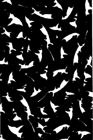
Fig. B 8.1 The upper central part of the picture shows a human face. The face can be recognized only with difficulty when looking at the picture for the first time (courtesy of H. Ritter)
We mentioned above properties of systems that cannot directly be traced back on a particular mechanism or a particular structure. Such properties are sometimes called emergent properties. As these seem to be important abilities, the question of emergence should be discussed briefly. The term emergence is often used when a property of a system comes "out of the blue," i. e., if we cannot understand why or how the property occurs, although we have the impression of understanding the properties of the elements of the system. In order to apply the concept of emergence, a definition of the term "emergent property" might be useful. According to Steels (1994b) , in an attempt to find an objective definition, a property is emergent if descriptive categories are needed to define it, which are not necessary to describe the behavior of the constituent components. A very simple example might be the occurrence of the resonance properties of a 2nd order system ( Part I – Chapter 4.9 ). In this case, the term resonance frequency is not necessary (or useful) for describing the behavior of a 1st order electrical system consisting of an ohmic resistor and a capacitor, or a system consisting of an ohmic resistor and an inductivity. But the term resonance is very helpful to describe the behavior of a system which contains all three elements. There is no single module in the system that produces the effect of resonance. Rather, this is produced by the cooperation of these elements. Therefore, this property does not exist on the level of the elements but only on the level of the complete system. This means that there are phenomena where, to understand them, one might be inclined to look for a particular module responsible for a particular property, although no such module exists. It might be argued that this property exist only "in the eye of the observer," i. e., that it is produced by our brain, but this is an epistemological question which will not be treated here. Other examples, more sophisticated than the electric oscillator, are the rolling waves in the Benard experiment, or the states occurring in a gas laser ( Haken 1973 ). In these cases, the occurrence of an emergent property is understood. A simple example in robotics might be the wall-following behavior of Pfeifer's robot (Fig. 16.6). A biological case is that some gait patterns in walking are not prespecified by a definite gait module, but "emerge" as a result of cooperation of leg controllers which cooperate via specific local rules ( Cruse 1990 ). Thus, although a gait pattern like a gallop immediately takes our eyes, there might be no specific gallop module in the brain of such an animal. It is sometimes assumed that the property of intelligence, which some systems appear to have, is also an emergent property. Similarly, the impression of an human observer that an animal (or, even more obviously, an animat), appears to have emotional states may manifest emergent properties. In the later case, the epistemological question mentioned above is even more difficult to answer.
When discussing the question of representations, we earlier discussed the idea of storing symbolic information. However, as mentioned, such a symbol may also only exist as an emergent phenomenon, and the distinction between symbolic and nonsymbolic information may be irrelevant at the level of the constituent elements. (The individual bit in the computer does not know whether it belongs to a symbol or not). An animat may well be regarded a symbol user because it exploits entities of the physical world (e.g., wall, corner) to which we would attach a symbol, although there is no corresponding symbolic representation in the "brain" of the animat.
In any case, these considerations should make clear that it is important to distinguish between the level of the observable behavior of an animal or an animat and the underlying mechanisms. There might even be more than two levels. This could be illustrated by slightly reformulating the classical question of Letvin and Maturana: what does the fly detector in the frog's retina tell the frog's brain? Does it say "there is a fly outside," or "start the catch reflex," or "there is an increased acetylcholine concentration at some synapses?" Of course, the sensors measure but do not interpret the world. However, the cooperation of the units of the whole system is such as to influence the human observer that he or she applies one of the "higher" interpretations.
Can we understand how the property of intelligence has evolved? There is an immense number of definitions of this term, and we do not intend to add another. It should, however, be clarified that there are two different ways of using this term, as an adverb and the nominal use. A system might be "intelligently designed," either by a constructor or by evolution, or it may itself have the capacity of intelligence. These two aspects might also be called species intelligence and individual intelligence. Sometimes, the first case is also called "hard-wired," although this term is misleading and will not be used here. Sometimes the term competence is proposed to distinguish species intelligence from nominal intelligence. Essential properties of a not just "competent," but "really" intelligent system might be the following. Such a system should sensibly react to novel situations, and find novel solutions to familiar situations. It should be capable of reasoning (i. e., finding a novel chain of inferences) and intelligent behavior should not be based on brute-force methods (i. e., exhaustive search) or on simple rules such as trial and error. In other words, cognition in the sense defined in Chapter 17 is a prerequisite for a system to be really intelligent.
Taking the discussion on emergent properties into account, one might assume that a module for intelligence does not necessarily exist, but that these properties may arise from the cooperation of simple elements. To approach this problem in more detail, the usually applied definitions, which tend to be subjective such as the Turing test (see Chapter 19 ), should be replaced by a more objective approach. In classic Artificial Intelligence a system was defined as intelligent, if it maximally applies the knowledge that it has (Newell: Steels 1994b ). To apply this definition to an animal or an animat, first the "subjective environment" of the system must be defined, meaning the part which can be investigated by its sensors, and the part in which it is admissible for the system to use its actuators, because an action can only be judged intelligent (or not) for a given subjective environment. Furthermore, the cost function, which should be minimized, has to be defined. Taking into account the biological view of considering systems which have to survive, a system might be called intelligent if "it maximizes the chances of self-preservation in a particular environment even if the environment changes" ( Steels 1994b ). This definition could also be applied to animats and was actually invented for this purpose. It no longer distinguishes between intelligence by design and individual intelligence, but only concentrates on the ability of the system to survive. This means that no distinction is made in principle, as to whether the system has acquired its knowledge during evolution or during learning as an individual.
Thus, the evolutionary series described earlier illustrates a series of systems with an increasing capability to survive and therefore with an increasing intelligence. There is a continuum, and each observer may introduce a threshold above which the systems might be called "intelligent" depending on his or her personal intuition.
The evolved versions of animats described earlier already showed activities as acting partly independent of actual sensory input, keeping a "goal in mind" and following it, although the system has to deal with disturbances, and although even the direct sensory contact is missing at some time. Learning systems can develop new modules and use them later during their "life." All these properties might be subsumed under the term prerational intelligence ( Cruse, Dean, Ritter, 1995 and Dean, Cruse, Ritter, 2000 ). Prerational intelligence is surely an emergent property, and it is an open question whether rational intelligence requires a special "rationality" module, or whether rationality, too, is an emergent property.
A system property is called emergent if there is no special module that is responsible for the appearance of such a property. Symbolic information, and the phenomenon of intelligence, at least prerational intelligence, may be examples of emergent properties.
In the last two chapters, different properties of animats have been discussed. Sometimes, specifically at the end of Chapter 17 , psychological terms have been used such as the system having emotions, expectations, and so on. These were, of course, as indicated by the inverted commas only used in a metaphorical sense for illustration, and not to mean that these animats actually have psychic states such as we experience by means of introspection, e. g., a sensation of pain, or being in an emotional state. The best one could say is that they behave as if they had such a state. However, this raises the question of whether such an artificial system could really have such states, and one could extend the question to phenomena such as our perception of the impression of consciousness or free will. An answer could be helpful in two aspects. If we could build such machines, it would not only help us to understand the important unsolved questions regarding what these phenomena are about but, with respect to application, if we assume that the occurrence of psychic states is coupled with higher mental capabilities, it might also help us to develop machines endowed with such capabilities.
As already described, machines can be built that give an observer the impression that they have internal states. Could an animat have something corresponding to a psychic state? Apart from asking more complicated questions, such as whether an animat could have consciousness or free will, we want to concentrate on the elementary, and more crucial question of whether, and under what conditions, an animat (or an animal) could have an internal impression (experience) at all, even of the simplest kind. In other words, is it possible that animals or animats experience the internal aspect as we do, or does the external aspect describe everything? For better clarification of the difference between internal and external aspects, we shall consider the phenomenon of pain. If a human subject touches a hot plate, he or she usually shows a fast withdrawal reflex and reports feeling pain. This is the external aspect of the observer (or third person's view). This observation could be described in more detail, if the neuronal activity of the subject could be investigated. But even if we assume that all neuronal details are known and a strict correlation (and a causal relation) between neuronal activities and the subject's report of feeling pain can be made, there is still a fundamental difference between this external aspect and the experience of "feeling pain." Even if the subject observes his or her own action potentials, this is not the pain felt. This internal aspect, based on the ability to feel, is also called the first person's view. Of course, a simple automaton could be constructed that shows a corresponding withdrawal reflex and expresses having felt pain: but we can be sure that there is no internal aspect in this case. That the latter is not necessary for the withdrawal reflex is already known for humans. The subjective impression of pain occurs some milliseconds after the motor reflex. When thinking of the internal aspect, we are often using the metaphor of a homunculus who observes the brain activities. However, this is a misleading metaphor. It transforms the situation into a kind of daily experience of the outside world. However, the inner aspect is something completely different, and any outside-world metaphor would probably be wrong. How can we decide whether a system really has an internal aspect? Is it only a special property of highly developed systems such as primates or even just humans?
According to Descartes, an absolutely certain decision as to whether a sensation is experienced can only be made by the organism itself. Only the subject is capable of experience by introspection, using his or her internal view, of feelings such as pain or joy. Whether other subjects have the same, or corresponding, conscious experiences, can only concluded by analogy. "Based on my own experience in the past I judge that he behaves as I would behave if I had this or that particular conscious experience. Therefore, I assume that he has the same conscious experience." However, this is an indirect conclusion. One can never have direct access to the experience of another subject. If one had full knowledge of all neuronal activities in the other subject's brain, and one could understand the causal sequences of the events in that brain, one could probably predict the experiences which the subject reports to feel at a particular moment; but even if one had the most detailed knowledge, it would always reflect the "external aspect." The knowledge of the observer is never the same as the experience of the subject. In human beings, an observer can by means of empathy, of course develop a good imagination of what is felt by another human and thus, in this sense, have more or less the same knowledge. This is not what is meant here, though. The content of knowledge may be the same, but the ontological nature of knowledge is different. To illustrate this difference, two possible misinterpretations will be mentioned. It is conceivable that someone believes an animal or an animat to experience feelings although this is not justified for somebody who, in the case of a robot, knows the simple structure of the animat. Conversely, we may not be prepared to attribute to a fly the experience of an internal aspect, although it may possibly experience it.
In philosophy, this dualism between the external and the internal aspect has been discussed intensively. One question has been whether a causal relationship between both worlds exists. Some argue that this dualism does not really exist, but only seems real. They assume that, in time, we will be accustomed to these views and will consider both the same, nondifferent in the sense of the two sides of a coin (mind-brain identity). Others have said, and still say, "ignorabimus," i. e., we will never understand this problem. A way to overcome this dualistic view might be as follows: One might argue that all the entities we experience, be they feelings like fear, or "hard facts" like reading a figure from the scale of a voltmeter, basically belong to the internal world. Although usually only the former entities are described as belonging to the internal world, actually the latter do so as well. We experience the view of the figure too. Therefore, one might argue that both worlds are not distinct sets, but that the external, "objective" world is a subset of the internal, subjective world, and not at all its dualistic counterpart.
How could we decide whether an entity belongs to the "objective" subset? Two speculative possibilities will be proposed. All the entities of the subjective world might be ordered along a line describing whether, when being recognized, they elicit empathy or not. (There is no clear-cut borderline: a tree might be emotionally loaded when providing a shadow in the heat, and may be much less so in other situations). Only in the latter case is the entity considered as an objective fact. The entities of the subjective world might also be ordered along another line, which, however, may be correlated with the first. Some entities can more easily be distinguished from each other than others. Therefore, the former may be countable and can be more easily attributed to symbols. These are the ones we call objective whereas the other items are called subjective. Taken together, this view leads to the assumption that there is a quantitative, maybe a qualitative, but no ontological difference between both "worlds."
Nevertheless, the following can be stated: although the true epistemological borderline for realizing the existence of an internal view runs between the observer and all other organisms, including other humans, it is generally accepted that all human beings have an internal view. This can be supported by the argument of structural identity. As other humans have principally the same hardware, they function principally in the same way, and therefore also experience the internal aspect. With respect to animals, the less developed these are in phylogenetic terms, the less people are prepared to concede there is an internal aspect. However, the reason underlying this view is that, for example, a dog can much better provide us with information concerning its internal state than an insect can. This is, of course, not a conclusive argument. The structural argument does not help here either because we do not know whether any other structures, e. g., in insect brains, allow for the existence of the internal aspect.
Even if we had full knowledge of the state of a human or an animal brain, we would be able to parallel events in the outer world (the world of the observer) and the inner world only by means of correlation. Such a correlation becomes less possible, the more the observed brain differs from a human brain. Thus, the question of whether an insect "experiences," as opposed to being a simple "reflex machine," is (probably) impossible to answer. This, of course, becomes even more of a problem, if an artificial system is to be judged in this way. In some cases, a simple robot can give the impression of having experience but knowing its interior circuits, one would not be prepared to admit that it has experience. An attempt to solve this problem was Turing's test; an observer talks to a partner via a keybord and a monitor. The observer does not know whether the partner is a human subject or an artificial system. If the observer decides that the partner is human, although it is an artificial system, this system (according to Turing) may be called intelligent, which in our context, includes the property of having an internal aspect. But even if a complicated machine could be built that succeeded in all Turing tests, we would still not know whether it really has experience in the sense of the internal aspect or not. On the other hand, no dog would pass a Turing test although most dog owners would consider that their dogs can experience internal aspects.
Another approach to this problem is the biological view. The capability to have an experience in the sense of the first person's view might or might not affect the fitness of the animal, its capability to survive. If it touches a hot plate, the above mentioned withdrawal reflex could work, irregardless of whether the subject feels pain or not. Is there an evolutionary advantage to this experience, to the existence of the internal aspect? In what sense is a system fitter, if it has the ability to "feel?" Is the internal view an advantage or just an epiphenomenon?
To avoid possible misunderstanding, the following should be stated: One surely has to assume that in living systems, and also in artificial ones, states may exist that correspond to some motivational state (seen from the external view), and that therefore structures and mechanisms may exist which, for example, have the function of controlling attention shift (see Maes model). However, it is completely open whether the phenomenon of an internal aspect is necessarily connected to the appearance of such structures. There are two theoretical possibilities. (a) The existence of an internal aspect is necessary in the sense that a phylogenetic advantage is coupled with this phenomenon. This would mean that special structures have developed during evolution which are responsible for the occurrence of the internal aspect. This means that, in principle, they could be copied for an artificial system. This would be very interesting for any applications because it would enable us to build machines having these advantages whatever they are. (b) Alternatively, the existence of an internal aspect is a pure epiphenomenon in the sense that there is no advantage with respect to evolution. On this assumption, the conscious I would only be an observer. Two problems are involved in this possibility: if the conscious I is only a (passive) observer, it means that the impression of free will can only be a delusion. If epiphenomenon means that there is no effect which can be observed from outside, it also means that this is no scientific hypothesis in the strict sense, because it cannot be tested.
Since, at this point, there seems to be no way of understanding the magic phenomenon of one's own internal aspect, we will, in the following, disregard it. Instead, we will concentrate on the external aspect only, i.e., we will ask under what conditions a subject may experience an internal aspect.
As mentioned earlier, one could imagine the brain as consisting of a number of modules which are responsible for specialized tasks. Many of these modules register inputs from the outer world and react to these signals. According to Minsky's ideas ( Minsky 1985 ), there are modules working on a lower level which detect the details of the environment (e. g. form and color of an obstacle). There may also be modules which are specialized in representing particular aspects of the world, e. g., position of distant objects or of parts of the body. From the latter, an internal model of the world could be constructed. Some module (perhaps most of them) detect the states of other modules and react to their signals. Some of them might obtain input from these internal world representations. The task of these modules is to determine possible future actions on the basis of this information, for example controlling the movement of the parts of the subject's own body through an obstacle-cluttered environment.
Can these considerations also be applied to machines? How could such circuits work? In the past, it was even doubted whether a machine was capable of anything more than purely reflexive responses to sensory inputs, such as pursuing a goal. However, as shown in Part I – Chapter 8 , a simple feedback system could do just this, holding a given value close to a goal (reference input) against various and unpredictable disturbances. As mentioned, animats already exist which have a simple explicit internal representation of the world and it is possible to build these animats with internal representations based on an modular architecture. Seen from the external aspect, those modules, which obtain input from the modules containing the world model, could be the locus where the whole system could "experience" the situation, in our example itself situated in a given environment. The system would therefore behave as if it really had an internal aspect. Whether it really does or not, cannot be answered. Nevertheless, we would like to speculate that the prerequisite for an "experiencing" system, i. e., a system with an internal aspect, is that modules exist which are able to view an inner representation of the world. One might further speculate that this is not only a necessary, but also a sufficient condition for a system to have an internal aspect.
Similarly, is it possible to think of a structure which shows the outer-aspect properties of a system having consciousness? The experience of feeling pain is a special and important event occurring in the consciousness. When we consider the phenomenon of consciousness generally, this is regarded as an experience to which several special properties can be attributed. Three important ones seem to mark this phenomenon. The first is the (i) "limitation" of consciousness: only very few items are conscious at a given time. It also seems (ii) that consciousness is occupied with the problem that is "most important" at the actual moment. This seems to help in enabling the whole system (iii) to concentrate on this important problem. Could these properties be implemented in an artificial system? These observations might be explained by the assumption that there is a module which detects problems, i. e., situations where two (or more) conflicting modules are highly excited. We can further assume that this problem-detecting module affects the system in such a way that the input to those conflicting modules remains high, so that any problem-solving module is constrained to deal with this problem. When another module, which surveys the entire situation, can only "see" the activities with the highest excitation, it "sees" only those types of information which seem to correspond to those which are in our consciousness; it refers to the most important problem of the moment; it contains only one problem, and the whole system concentrates on this problem as long as it is unsolved (and is still the most important one). (See Cruse 1979 for a more detailed discussion). As it is generally not a problem to develop machines with internal models and modules which observe only the most important problem, one could assume that such a machine presents the external aspect of a system endowed with consciousness. However, as mentioned above, it is completely unclear, how one could test whether this machine really has an experience, or an internal view, other than by the very indirect tests like those proposed by Turing.
We believe that eventually machines will be built that - from the standpoint of the external view - will behave as if they had emotions, or motivations, and consciousness. Whether they will really have them in the sense of an internal aspect, strictly speaking, will (probably) never be known. Nevertheless, on the basis of an analog conclusion, we may ascribe to them an internal view; we do this now with respect to other humans, some of us to a dog, some even to a frog, and possibly a bee. Such a machine can take a position anywhere in this series, depending on its subjective similarity with the self-image of the observer.
One possible interpretation concerning the nature of the internal aspect is that there exist structures (the modules mentioned) which have an evolutionary advantage, but that the phenomenon of experience as such (e.g., of pain) can be considered an epiphenomenon which, by itself, has no particular advantage in an evolutionary sense. An internal view possibly appears whenever certain structural conditions are fulfilled. As mentioned above, the capability to experience an internal view may be based on the ability to view internal world models and may have developed quite early in evolution.
If the above mentioned speculations are correct, i. e., that a machine could have feelings and even consciousness, one may further ask whether a machine could also have free will. What does is mean for a human to have free will? We do not know what (free) will is, but we do experience it. If we have to make a decision, we do not have the impression that the result is already fixed beforehand, rather that we make it during the process, and that we are responsible for the result. This reflects the internal aspect. However, considering such a system from outside, the behavior seems to be determined by sensory input (plus internal systems including memory) and, possibly, random effects produced, for example, by chaotic properties. Insofar, there seems to be no basic difference to a machine. But even though one may accept this view, one still has the introspective impression of having a free will. Can a deterministic system have a free will and therefore be responsible for its actions? To some, this seems to be a contradiction, but reflects the different realities of the internal and the external aspect. This is similar to when we see the sun rise in the morning and move across the sky during the day, although we "know" that it is not the sun which moves. Similarly, we speak of psychosomatic effects, although many of us are sure that there is no literal influence of the "psychic" on the physical domain other than our ideas. We mix items of the external and the internal aspect, which is, strictly speaking, not permissible, but comfortable because it is complicated to always describe the "real" relationship. Thus, we will continue using the term free will not only because it corresponds to our internal experience, but also because it is a simple and important concept with respect to our whole cultural life. The loss of this concept could lead to misunderstandings which might produce a number of social problems. The concept that humans have a free will and are thus responsible for their actions and therefore the concept of moral depth, would lose its essential foundation. If this became accepted it would nevertheless be necessary to formulate social rules, such as laws and fines, as if free will existed, to avoid social disaster. Then, the mental modules would have to take into account the corresponding reactions of the world, and in this way, sensible social existence would still be possible. This view is actually already common, as it has long been in jurisdiction: fines represent a means of preventing crimes and not a means of atoning for moral debt. However, this line of argument is complicated and hence less comprehensible. Life would therefore not be easier, if this knowledge were to be accepted by the human community. Another problem which might hamper the acceptance of these concepts is that they will be understood by many as questioning the idea of human self-understanding and of human dignity. We are, however, quite confident with respect to overcoming the latter problem because we easily survived three other attacks on these ideas, first, the Copernican revolution, second, the Darwinian revolution, and third, Freuds detection of the contribution of unconsciousness.
The elementary question discussed is whether animals or animals could have an internal experience as a human can experience this by observing him or herself. The difference between the internal and the external aspect can be made clear by considering the difference between feeling pain and looking at one's own neuronal activity correlated with this experience. Whether an insect (or an animal) "experiences" as opposed to being a simple "reflex machine" without an internal aspect, is (probably) impossible to answer. However, the argument of structural analogy, which can be used to accept the existence of an internal aspect in other humans except oneself, might, after further studies, in future also allow for conclusions with respect of other animals and possibly animats.
Abramowitz, M., Stegun, I. (1965): Handbook of Mathematical Functions. Dover Publications, New York
Adam, D., Windhorst, U., Inbar, G.F. (1978): The effects of recurrent inhibition on the cross-correlated firing pattern of motoneurons (and their relation to signal transmission in the spinal cord-muscle channel). Biol. Cybernetics 29, 229-235
Amari, S. (1967): Theory of adaptive pattern classifiers. IEEE Trans., EC-16, No. 3, 299-307
Amari, S. (1968): Geometrical theory of information (in Japanese). Kyoritsu-Shuppan, Tokyo
Amari, S., Arbib, M.A. (1982): Competition and Cooperation in Neural Nets. Springer Lecture Notes in Biomathematics Nr 45
Arbib, M.A. (1995): Schema theory. In: M.A. Arbib (ed.) The Handbook of Brain Theory and Neural Networks. MIT Press, Bradford Book, Cambridge, Mass, 1995
Baldi, P., Heiligenberg, J.M. (1988): How sensory maps could enhance resolution through ordered arrangements of broadly tuned receivers. Biol. Cybern. 59,313-318
Barto, A.G., Sutton, R.S., Brouwer, P.S. (1981): Associative search network: a reinforcement learning associative memory. Biol. Cybern. 40, 201 -211
Barto, A.G., Sutton, A.G., Watkins, C. (1990): Sequential decision problems and neural networks. In: M. Gabriel, J.W. Moore (eds.) Advances in neural information processing systems. Morgan Kaufmann 1990, 686-693
Bässler, U. (1983): Neural basis of elementary behavior in stick insects. Springer, Berlin, Heidelberg, New York
Bässler, U. (1993): The femur-tibia control system of stick insects - a model system for the study of the neural basis of joint control. Brain Res. Rev. 18, 207-226
Bechtel, W., Abrahamsen, A.A. (1990): Connectionism and the mind: an introduction to parallel processing in networks. Basil Blackwell, Oxford
Beckers, R., Deneubourg, J.L, Goss, S. (1992): Trails and U-turns in the selection of a path by the ant Lasius niger. J. of Theor. Biol. 159, 397-415
Brooks, R.A. (1986): A robust layered control system for a mobile robot. J. Robotics and Automation 2, 14-23
Brooks, R.A. (1989): A robot that walks: emergent behaviours from a carefully evolved network. Neural Computation I, 253-262
Cabanac, M. (1992): Pleasure: the common currency. J. Theor. Biol. 155, 173-200
Camazine, S., Deneubourg, J.-L., Franks, N. R., Sneyd, J., Theraulaz, G., Bonabeau, E. (2003) Self-organization in biological systems. Princeton Univ. Press, Princeton
Carpenter, G.A., Grossberg, S. (1987): A massively parallel architecture for a self-organizing neural pattern recognition machine. Computer Vision, Graphics, and Image Processing 37, 54-115
Chapman, K.M.. Smith, R.S. (1963): A linear transfer function underlying impulse frequency modulation in a cockroach mechanoreceptor. Nature 197, 699-700
Clynes, M. (1968): Biocybernetic principles and dynamic asymmetry: unidirectional rate sensitivity. In: H. Drischel (ed.) Biokybernetik. Vol. 1, Fischer, Jena 29-49
Cruse, H. (1979): Modellvorstellungen zu Bewußtseinsvorgängen. Naturw. Rdschau 32, 45-54
Cruse, H. (1981): Biologische Kybernetik. Verlag Chemie. Weinheim, Deerfield Beach, Basel
Cruse, H. (1990): What mechanisms coordinate leg movement in walking arthropods? Trends in Neurosciences 13, 1990, 15-21
Cruse, H. (2002). Landmark-based navigation. Biol. Cybernetics 88, 425-437
Cruse, H., Bartling, Ch., Kindermann, Th. (1995): Highpass filtered positive feedback: decentralized control of cooperation. In: F. Moran, A. Moreno, J.J. Merelo, P. Chacon (eds.) Advances in Artificial Life. Springer, 668-678
Cruse, H., Dean, J., Heuer, H., Schmidt, R.A. (1990): Utilisation of sensory information for motor control. In: 0. Neumann, W. Prinz (eds.) Relationships between perception and action. Springer, Berlin, 43-79
Cruse, H., Dean, J., Ritter, H. (1995): Prärationale Intelligenz. Spektrum d. Wiss. 111-115
Daugman, J.G. (1980): Two-dimensional spectral analysis of cortical receptive field profiles. Vision Res. 20, 847, 856
Daugman, J.H. (1988): Complete discrete 2-D Gabor transforms by neural networks for image analysis and compression. IEEE Transact. on acoustics, speech, and signal processing. 36, 1169-119
Dean, J. (1990): Coding proprioceptive information to control movement to a target: simulation with a simple neural network. Biol. Cybern. 63, 115-120
Dean, J., Cruse, H., and Ritter, H. (2000): Prerational Intelligence: Interdisciplinary perspectives on the behavior of natural and artificial systems. Kluwer Press, Dordrecht
Deneubourg, J.L, Goss, S. (1989): Collective patterns and decision making. Ethology, Ecology and Evolution 1, 295-311
Dijkstra, S., Denier van der Gon, J.J. (1973): An analog computer study of fast isolated movements. Kybernetik 12,102 -110
DiStefano, 111, Joseph J., Stubberud, Allen R., Williams, Ivan J. (1967): Theory and Problems of Feedback and Control Systems with Applications to the Engineering, Physical, and Life Sciences. McGraw Hill, New York, St. Louis, San Francisco, Toronto, Sydney
Eckhorn, R., Bauer, R., Jordan, W., Brosch, M., Kruse, W., Munk, M., Reitboeck, H.J. (1988): Coherent oscillations: a mechanism of feature linking in the visual cortex? Multiple electrode and correlation analysis in the cat. Biol. Cybernetics 60, 121 - 130
Eibl-Eibesfeldt, I. (1980): Jumping on the sociobiology bandwagon. The Behavioral and Brain Sciences 3, 631-636
Elman, J.L. (1990): Finding structure in time. Cognitive Science 14, 179-211
Engel, A.K., König, P., Kreiter. A.K., Schillen, TB., Singer, W. (1992): Temporal coding in the visual cortex: new vistas on integration in the nervous system. Trends in Neurosciences 15, 218-226
Exner, S. (1894): Entwurf einer physiologischen Erklärung der psychischen Erscheinungen. 1. Ted. Deuticke, Leipzig, 37-140
Fahlman, S.E., Lebiere, C. (1990): The cascade correlation learning architecture. In: D.S. Touretzky (ed.) Advances in neural information processing systems 2. Morgan Kaufman Pub. San Mateo, CA, 524-532
Fenner, F.J., Gibbs, E.P.J., Murphy, EA., Rott, R., Studdert, M.J., White, D.O. (1993): Veterinary Virology. Academic Press. San Diego, New York, Boston
Franceschini, N., Riehle, A., Le Nestour, A. (1989): Directionally selective motion detection by insect neurons. In: Stavenga, Hardie (eds.) Facets of Vision. Springer, Berlin, Heidelberg, 360-390
Fukushima, K. (1975): Cognitron: a self-organizing multilayered neural network. Biol. Cybern. 20, 121-136
Fukushima, K. (1980): Neocognitron: a self-organizing neural network model for a mechanism of pattern recognition unaffected by shift in position. Biol. Cybern. 36,193-202
Haken, H. (ed.) (1973): Synergetik. Teubner, Stuttgart
Hartmann, G., Wehner, R. (1995): The ant's path integration system: a neural architecture. Biol. Cybern. 73, 483-497
Hassenstein, B. (1958 a): Über die Wahrnehmung der Bewegung von Figuren und unregelmäßigen Helligkeitsmustern am Rüsselkäfer Chlorophanus viridis. Zeitschrift für vergleichende Physiologie 40, 556-592
Hassenstein, B.(1958 b): Die Stärke von optokinetischen Reaktionen auf verschiedene Mustergeschwindigkeiten (bei Chlorophanus viridis). Z. Naturforschg. 12 b, 1-6
Hassenstein, B. (1959): Optokinetische Wirksamkeit bewegter periodischer Muster (nach Messungen am Rüsselkäfer Chlorophanus viridis). Z. Naturforschg. 14b, 659-674
Hassenstein, B. (1966): Kybernetik und biologische Forschung. Handbuch der Biologie, vol. 1/2, pp. 629-719. Akademische Verlagsgesellschaft Athenaion. Frankfurt/M.
Hassenstein, B. (1971): Information and control in the living organism. Chapman and Hall, London
Hassenstein, B., Reichardt, W. (1953): Der Schluß von den Reiz-Reaktions-Funktionen auf System-Strukturen. Z. Naturforsch. 86, 518-524
Hassenstein, B., Reichardt, W. (1956): Systemtheoretische Analyse der Zeit-, Reihenfolgen- und Vorzeichenauswertung bei der Bewegungsperzeption des Rüsselkäfers Chlorophanus. Z. Naturforschg. 11 b, 513-524
Hebb, D.O. (1949): The organization of behavior. Wiley, New York
Heisenberg, M., Wolf, R(1988): Reafferent control of optomotor yaw torque in Drosophilia melanogaster. J. Comp. Physiol. 163:373-388
Hertz, J., Krogh, A., Palmer, R.G. (1991): Introduction to the theory of neural computation. Addison-Wesley Pub., Redwood City
Hinton, G.E., McClelland, J.L., Rumelhart, D.E. (1986): Distributed representation. In: D.E. Rumelhart, J.L. McClelland (eds.) Parallel Distributed Processing, Vol. 1, MIT Press, Cambridge MA, 77-109
Holland, J.H. (1975): Adaptation in natural and artificial systems. Univ. of Michigan Press (2nd edition MIT Press, 1992)
Holst, E.v. (1950a): Die Arbeitsweise des Statolithenapparates bei Fischen. Zeitschr. Vergl. Physiol. 32, 60-120
Holst, E.v. (1950b): Die Tätigkeit des Statolithenapparats im Wirbeltierlabyrinth. Naturwissenschaften 37, 265-272
Holst, E.v. (1957): Aktive Leistungen der menschlichen Gesichtswahrnehmung. Studium Generale 10, 231-243
Holst, E.v., Mittelstaedt, H. (1950): Das Reafferenzprinzip: Wechselwirkungen zwischen Zentralnervensystem und Peripherie. Naturwissenschaften 37, 464-476
Hopfield, J.J. (1982): Neural networks and physical systems with emergent collective computational abilities. Proc. Natl. Acad. Sci. 79, 2554-2558
Hopfield, J.J. (1984): Neurons with graded response have collective computational properties like those of two-state neurons. Proc. Natl. Acad. Sci. 81, 3088-3092
Hopfield, J.J., Tank, D.W. (1985): "Neural" computation of decisions in optimization problems. Biol. Cybern. 52, 141-152
Iles, J.F., Pearson, K.G. (1971 ): Coxal depressor muscles of the cockroach and the role of peripheral inhibition. J. Exp. Biol. 55,151 -164
Jacobs, R.A., Jordan, M.1., Nowlan, S.J., Hinton, G.E. (1991): Adaptive mixtures of local experts. Neural Computation 3, 79-87
Jaeger, H., Haas, H. (2004): Harnessing Nonlinearity: Predicting Chaotic Systems and Saving Energy in Wireless Communication. Science, April 2, 2004, 78-80. [Preprint including supplementary material: http://www.faculty.iu-bremen.de/hjaeger/pubs/ESNScience04.pdf ]
Jordan, M.L (1986): Attractor dynamics and parallelism in a connectionist sequential machine. In: Proceedings of the eighth annual conference of the cognitive science society. (Amherst 1986) Hillsdale, Earlbaum, 531 - 546
Jordan, M.L (1990): Motor learning and the degrees of freedom problem. In: M. Jeannerod (ed.) Attention and Performance XIII. Hillsdale, NJ, Earlbaum, 796-836
Jordan, M.L, Jacobs, R.A. (1992): Hierarchies of adaptive experts. In: J. Moody, S. Hanson, & R. Lippmann, (eds.) Neural Information Systems, 4. Morgan Kaufmann, San Mateo, CA
Jones, W.P., Hoskins, J. (1987): Backpropagation: a generalized delta learning rule. Byte 155-162
Kandel, E.R.. Schwartz, J.H., Jessel, T.M. (2000): Principles of neural science. Elsevier, New York, Amsterdam, Oxford
Kawato, M., Gomi, H. (1992): The cerebellum and VOR/ OKR learning model. Trends in Neurosciences 15,455 - 453
Kindermann, Th., Cruse, H., Dautenhahn, K(1996): A fast, three layered neural network for path finding. Network: Computation in Neural Systems 7, 423-436
Koch, U.T., Bässler, U., Brunner, M. (1989): Non-spiking neurons suppress fluctuations in small networks. Biol. Cybern. 62, 75-81
Kohonen, T. (1982): Self-organized formation of topologically correct feature maps. Biol. Cybern. 43, 59-69
Kohonen, T. (1988): An introduction to neural computing. Neural Networks 1, 3-16
Kohonen, T. (1989): Self-organization and associative memory. Springer Series in Information Sciences. Springer Verlag, 3rd edition
Koza. J.R. (1992): Genetic programming: A paradigm for genetically breeding computer population of computer programs to solve problems. MIT Press, Cambridge MA
Kühn, S., Beyn, W.-J., Cruse, H. Modeling memory function with recurrent neural networks consisting of Input Compensation units. I. Static Situations. (submitted)
Kühn, S., Cruse, H. Modelling memory function with recurrent neural networks consisting of Input Compensation units. II. Dynamic Situations. (submitted)
Le Cun, Y. (1985): Line procedure d'apprendissage pour reseau a seuil assymetrique. In: Cognitiva 85: A la frontiere de I'intelligence artificielle des sciences de la connaissance des neurosciences. Paris 1985, 599604. Paris CESTA
Levin, E. (1990): A recurrent network: limitations and training. Neural Networks 3, 641-650
Linder, C. (2005) Self-organization in a simple task of motor control based on spatial encoding. Adaptive Behavior 13, 189-209
Littmann, E., Ritter, H. (1993): Generalization abilities of cascade network architectures. In C.L. Giles, S.J. Hanson, J.D. Cowan (eds.) Advances in neural information processing systems 5. Morgan Kaufman Pub., San Mateo, CA, 188-195
Lorenz, K. (1950): The comparative method in studying innate behavior patterns. Symp. Soc. Exp. Biol. 221 - 268
Maass, W., Natschläger, T. and Markram. H. (2002): Real-time computing without stable states: A new framework for neural computation based on perturbations. Neural Computation, 14(11):2531-2560 http://www.lsm.tugraz.at/papers/lsm-nc-130.pdf
Maes, P. (1991): A bottom-up mechanism for behavior selection in an artificial creature. In: J.A. Meyer, S.W. Wilson (eds.) From animals to animats. Bradford Book, MIT Press, Cambridge Mass, London, 238-246
von der Malsburg, Ch. (1973): Self-organization of oriented sensitive cells in the striate cortex. Kybernetik 14, 85-100
von der Malsburg, Ch. (1981): The correlation theory of brain function, Internal report 81-2, Göttingen, Germany: Max Planck Institut fur Biophysikalische Chemie. Reprinted in: Models of Neural Networks (K. Schulten, H.J. van Hemmen, eds.) Springer, 1994
von der Malsburg, Ch., Buhmann, J. (1992): Sensory segmentation with coupled neural oscillators. Biol. Cybern. 67, 233-242
Marmarelis, P.Z., Marmarelis, V.Z. (1978): Analysis of physiological systems: the white noise approach. Plenum Press, New York
Martinetz, T., Ritter, H., Schulten, K. (1990): Three-dimensional Neural Net for Learning Visuomotor-Coordination of a Robot Arm. IEEE-Transact. on Neural Networks 1,131-136
McFarland. D., Bösser, Th. (1993): Intelligent behavior in animals and robots. Bradford Book, MIT Press, Cambridge MA
Meinhardt, H. (1995): The algorithmic beauty of sea shells. Springer, Heidelberg
Milhorn, H.T. (1966): The application of control theory to physiological systems. Saunders, Philadelphia
Milsum, IT. (1966): Biological control systems analysis. McGraw Hill, New York
Minsky, M. (1985): The society of mind. Simon and Schuster, New York
Minsky, M.L., Papert, S.A. (1969): Perceptrons. MIT Press, Cambridge
Möhl, B. (1989): "Biological noise" and plasticity of sensorimotor pathways in the locust flight system. J. comp. Physiol. A 166, 75 -82
Möhl, B. (1993): The role on proprioception for motor learning in locust flight. J. Comp. Physiol. A 172, 325-332
Nauck D, Klawonn F, Borgelt C, Kruse R (2003) Neuronale Netze und Fuzzy Systeme. Braunschweig/ Wiesbaden: Vieweg-Verlag.
Oppelt, W. (1972): Kleines Handbuch technischer Regelvorgange. Verlag Chemie, Weinheim
Pfeifer, R. (1995): Cognition - perspectives from autonomous agents. Robotics and Autonomous Systems 15, 47-69
Pfeifer, R., and Verschure, P.F.M.J. (1992): Distributed adaptive control: a paradigm for designing autonomous agents. In: Towards a practice of autonomous systems: Proc. of the First European Conference on Artificial Life. MIT Press, Cambridge, Mass. 21-30
Pichler, J., Strauss, R. (1993): Altered spatio-temporal orientation in ellipsoid-body-open, a structural central complex mutant of Drosophila melanogaster. In: Elsner, N., Heisenberg, M. (eds.) Gene, Brain, Behavior. Proceedings of the 21st Göttingen Neurobiology Conference. p. 813. Stuttgart, Thieme
Ratliff, E (1965): Mach Bands: Quantitative Studies on Neural Networks in the Retina. Holden-Day, San Francisco, London, Amsterdam
Rechenberg, L (1973): Evolutionsstrategie: Optimierung technischer Systeme nach Prinzipien der biologischen Evolution. Fromman-Holzboog. Stuttgart
Reichardt, W. (1957): Autokorrelationsauswertung als Funktionsprinzip des Zentralnervensystems. Z. Naturforsch. 12 b, 448 -457
Reichardt, W. (1973): Musterinduzierte Flugorientierung der Fliege Musca domestica. Naturwissenschaften 60, 122-138
Reichardt, W., MacGinitie, G. (1962): Zur Theorie der lateralen Inhibition. Kybernetik 1, 155-165
Riedmiller, M., Braun, H. (1993): A direct adaptive method for faster backpropagation learning: the RPROP Algorithm. Proceedings of the IEEE Int. Conf. on Neural Networks (IBNN), 586-591
Ritter, H., Kohonen, T. (1989): Self-Organizing Semantic Maps. Biol. Cybern. 61, 241-254
Ritter, H., Martinez, T., Schulten, K. (1989): Topology conserving maps for learning visuomotor coordination. Neural Networks 2, 159-168
Ritter, H., Martinetz, Th., Schulten, K. (1992): Neural Computation and Self-organizing Maps. Addison Wesley, 1 st revised english edition
Rosenblatt, E (1958): The perceptron: a probabilistic model for information storage and organization in the brain. Psychol. Rev. 65, 386-408
Rumelhart, D.E., Hinton, G.E., Williams, R.J. (1986): Learning internal representations by back-propagating errors. Nature 323, 533-536
Rumelhart, D.E., McClelland, J.L. (1986): Parallel Distributed Processing, Vol. 1, Bradford Book, MIT Press, Cambridge Mass, London
Schmidt, R. E. (1972): Grundriß der Neurophysiologie. Springer, Berlin, Heidelberg, New York
Schmidt, R. E. (1973): Grundriß der Sinnesphysiologie. Springer, Berlin, Heidelberg, New York
Schöner, G. (1991): Dynamic theory of action-perception patterns: the "moving room" paradigm. Biol. Cybern. 64, 455-462
Sejnowski, T. J., Tesauro, G. (1989): The Hebb rule for synaptic plasticity: algorithms and implementations. In: Byrne, J.H., Berry, W.O. (eds.) Neural models of plasticity: Experimental and theoretical approaches., Academic Press, pp. 94-103
Spekreijse, H., Oosting, H. (1970): Linearizing: a method for analysing and synthesizing nonlinear systems. Kybernetik 7, 22-31
Sperry, R. W. (1950): Neural basis of the spontaneous optokinetic response produced by visual inversion. J. Comp. Psychol. 43, 482-499
Steels, L. (1994a): Emergent functionality in robotic agents through on-line evolution. In: R. Brooks, P. Maes (eds.) Proceedings of the IV. MIT Press, Cambridge MA
Steels, L. (1994b): The artificial life roots of artificial intelligence. Artificial Life 1, 75-110
Steil, J.J. (1999) Input-Output Stability of Recurrent Neural Networks. Göttingen: Cuvillier Verlag.
Stein, R.B. (1974): Peripheral control of movement. Physiol. Rev. 54, 215-243
Steinbuch, K. (1961): Die Lernmatrix. Kybernetik 1, 36-45
Steinkühler, U., Cruse, H. (1998): A holistic model for an internal representation to control the movement of a manipulator with redundant degrees of freedom. Biol. Cybernetics 79, 457-466
Tani J, Nolfi S (1999) Learning to perceive the world articulated: an approach for hierarchical learning in sensory-motor systems. Neural Networks 12: 1131-1141.
Tank, D.W., Hopfield, J.J. (1987): Collective computation in neuron-like circuits. Scientific American 257, 104
Thorson, J. (1966): Small signal analysis of a visual reflex in the locust 11. Frequency dependence. Kybernetik 3, 53-66
Varju, D. (1962): Vergleich zweier Modelle für laterale Inhibition. Kybernetik 1, 200-208
Varju, D. (1965): On the theory of lateral Inhibition. Consiglio nazionale delle Ricerche, Rome, 1-26
Varju, D. (1977): Systemtheorie. Springer, Berlin, Heidelberg, New York
Varju, D. (1990): A note on the reafference principle. Biol. Cybern. 63, 315-323
Wagner, R. (1960): Über Regelung von Muskelkraft und Bewegungsgeschwindigkeit bei der Willkürbewegung. Z. Biol. 111, 449-478
Wehner, R. (1987): "Matched filters" - neural models of the external world. J. Comp. Physiol. A 161, 511-531
Werbos, P.J. (1974): Beyond regression: new tools for prediction and analysis in the behavioral sciences. Ph.D. Thesis, Harvard University
Williams, R.J. (1992): Simple statistical gradient-following algorithms for connectionist reinforcement learning. Machine Learning 8, 229-256
Willshaw, D.J., von der Malsburg, C. (1976): How patterned neural connections can be set up by self-organization. Proceedings of the Royal Society of London B 194, 431-445
Wilson, S.W. (1987): Classifier systems and the animat problem. Machine Learning 2,199 -228
Wolpert, D.M., Kawato, M. (1998): Multiple paired forward and inverse models for motor control. Neural Networks 11, 1317-1329
License
Any party may pass on this Work by electronic means and make it available for download under the terms and conditions of the Digital Peer Publishing License. The text of the license may be accessed and retrieved via Internet at http://www.dipp.nrw.de/lizenzen/dppl/dppl/DPPL_v2_en_06-2004.html

