
Document Actions
Neural Networks as Cybernetic Systems – Part 1
3rd and revised edition
Department of Biological Cybernetics, Bielefeld University, Universitätsstraße 25, 33615 Bielefeld, Germanyurn:nbn:de:0009-3-19884
Keywords: cybernetics, neurosciences, models, simulation, systems theory, ANN, neural networks
The task of a neuronal system is to guide an organism through a changing environment and to help it to survive under varying conditions. These neuronal systems are probably the most complicated systems developed by nature. They provide the basis for a broad range of issues, ranging from simple reflex actions to very complex, and so far unexplained, phenomena such as consciousness, for example. Although, during this century, a great amount of information on neural systems has been collected, a deeper understanding of the functioning of neural systems is still lacking. The situation appears to be so difficult that some skeptics speak of a crisis of the experimentalist. They argue that to continue to accumulate knowledge of further details will not help to understand the basic principles on which neural systems rely. The problem is that neuronal systems are too complicated to be understood by intuition when only the individual units, the neurons, are investigated. A better understanding could be gained, however, if the work of the experimentalist is paralleled and supported by theoretical approaches. An important theoretical tool is to develop quantitative models of systems that consist of a number of neurons. By means of proposing such models which, by definition, are simplified versions or representations of the real systems, comprehension of the properties of the more complicated, real systems might be facilitated.
The degree of simplification of such models or, in other words, the level of abstraction may, of course, be different. This text gives an introduction to two such approaches that will enable us to develop such models on two levels. A more traditional approach to developing models of such systems is provided by systems theory. Other terms of similar meaning are cybernetics or control theory. As the basic elements used for models in systems theory are known as filters (which will be described in detail later) the term filter theory is also used.
Systems theory was originally developed for electrical engineering. It allows us to consider a system on a very abstract level, to completely neglect the real physical construction, and to consider only the input-output properties of the system. Therefore, a system (in terms of systems theory) has to have input channels and output channels that receive and produce values. One important property is that these values can vary with time and can therefore be described by time functions. The main interest of the systems theory approach, therefore, concerns the observation of dynamic processes, i. e., the relation of time-dependent input and output functions. Examples of such systems could be an electrical system, consisting of resistors and capacitors as shown in Figure 1.1, or a mechanical system comprising a pendulum and a spring (Fig. 1.2). In the first case, input and output functions are the voltage values ui and uo. In the second case, the functions describe the position of the spring lever, x(t), and the pendulum, y(t), respectively. An example of a biological system would be a population, the size of which (output) depends on the amount of food provided (input). Examples of neuron-based systems are reflex reactions to varying sensory inputs. A classic example is the optomotor response that occurs in many animals and has been intensively investigated for insects by Hassenstein and Reichardt and co-workers in the 1950s and 60s (Hassenstein 1958 a, b, 1959: Hassenstein and Reichardt 1956; Reichardt 1957,1973).
Although the systems theory approach is a powerful tool that can also be applied to the investigation of individual neurons, usually it is used for model systems far removed from the neuronal level. However, earlier in the field of biological cybernetics, models were considered where the elements correspond to neuron-like ones, albeit extremely simplified. This approach has gained large momentum during the last 10 years, and is now known by terms such as artificial neural networks, massive parallel computation, or connectionist systems. Both fields, although sharing common interests and not included in the term cybernetics by accident, have developed separately, as demonstrated by the fact that they are covered in separate textbooks. With respect to the investigation of brain function, both fields overlap strongly, and differences are of quantitative rather than qualitative nature. In this text, an attempt is made to combine the treatment of both fields with the aim of showing that results obtained in one field can be applied fruitfully to the other, forming a common approach that might be called neural cybernetics.
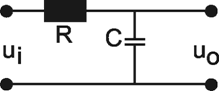
Fig. 1.1 An example of an electric system containing an resistor R, and a capacitor C. ui input voltage, uo output voltage
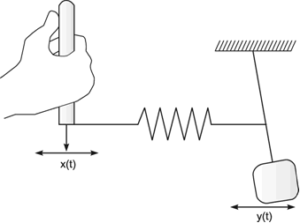
Fig.1.2 An example of a mechanical system consisting of an inert pendulum and a spring. Input function x(t) and output function y(t) describe the position of the lever and the pendulum, respectively
One difference between the models in each field is that in typical systems theory models the information flow is concentrated in a small number of channels (generally in the range between 1 and 5), whereas in a neural net this number is high (e. g., 10 - 105 or more). A second difference is that, with very few exceptions, the neural net approach has, up to now, considered only the static properties of such systems. Since in biological neural networks the dynamic properties seem to be crucial, the consideration of static systems is, of course, a good starting point: but unless dynamics are taken into account, such investigations miss a very important point. This is the main subject of systems theory, but neural nets with dynamic properties do exist in the form of recurrent nets.
To combine both approaches, we begin with classic systems theory, describing properties of basic linear filters, of simple nonlinear elements and of simple recurrent systems (systems with feedback loops). Then, the properties of simple, though massively parallel, feed-forward networks will be discussed, followed by the consideration of massively parallel recurrent networks. The next section will discuss different methods of influencing the properties of such massively parallel systems by "learning." Finally, some more-structured networks are discussed, which consists of different subnetworks ("agents"). The important question here is how the cooperation of such agents could be organized.
All of these models can be helpful to the experimentalist in two ways. One task of developing such a model-be it a systems theory (filter) model or a "neuronal" model-would be to provide a concise description of the results of an experimental investigation. The second task, at least as important as the first, is to form a quantitative hypothesis concerning the structure of the system. This hypothesis could provide predictions regarding the behavior of the biological system in new experiments and could therefore be of heuristic value.
Modeling is an important scientific tool, in particular for the investigation of such complex systems as biological neural networks (BNN). Two approaches will be considered: (i) the methods of system theory or cybernetics that treat systems as having a small number of information channels and therefore consider such systems on a more abstract level, and (ii) the artificial neural networks (ANN) approach which reflects the fact that a great number of parallel channels are typical for BNNs.
A system, in terms of systems theory, can be symbolized quite simply by a "black box" (Fig. 1.3a) with input and output channels. The input value is described by an input function x(t), the output value by an output function y(t), both depending on time t. If one was able to look inside the black box, the system might consist of a number of subsystems which are connected in different ways (e. g., Fig. 1.3b). One aim of this approach is to enable conclusions to be reached concerning the internal structure of the system. In the symbols used throughout this text, an arrow shows the direction of signal flow in each channel. Each channel symbolizes a value which is transported along the line without delay and without being changed in any way. A box means that the incoming values are changed. In other words, calculations are done only within a box. Summation of two input values is often shown by the symbol given in Fig. 1.4a (right side) or, in particular if there are more than two input channels, by a circle containing the summation symbol Σ (Fig. 1.4a, left). Figure 1.4b shows two symbols for subtraction. Multiplication of two (or more) input values is shown by a circle containing a dot or the symbol Π (Fig. 1.4c). The simplest calculation is the multiplication with a constant w. This is often symbolized by writing w within the box (Fig. 1.4d, right). Another possibility, mostly used when plotting massively parallel systems, is to write the multiplication factor w beside the arrowhead (Fig. 1.4d, left).
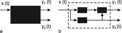
Fig. 1.3 Schematic representation of a system. (a) black box. (b) view into the black box. x(t) input function, y1(t),y2(t) output functions
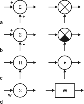
Fig. 1.4 Symbols used for (a) summation, (b) subtraction, and (c) multiplication of two (or more) input values and (d) for multiplication with a constant value
We can distinguish between linear and nonlinear systems. A system is considered linear if the following input-output relations are valid. If y1 is the output value belonging to the input value x1, and y2 that to the input value x2, the input value (x1 + x2) should produce the output value (y1 + y2). In other words, this means that the output must be proportional to the input. If a system does not meet these conditions, we have a nonlinear system.
This will be illustrated in Figure 1.5 by two selected examples. To begin with, Figure 1.5a shows the response to a step-like input function. If the input function rises sharply from the value zero to the value x, within this system the output function reaches the value y after a certain temporal delay. If the amplitude of the input function is doubled to 2 x, the values of the output function must be doubled, too, in case of a linear system (Fig. 1.5b, continuous line). If, however, the output function (y* ≠ 2y) shown in Figure 1.5b with a dashed line were achieved, it would be a nonlinear system.
Nonlinear properties occur, for example, if two channels are multiplied or if nonlinear characteristics occur within the system (see Chapter 5 ). Although the majority of all real systems (in particular, biological systems) are nonlinear in nature, we shall start with linear systems in Chapters 3 and 4 . This is due to the fact that, so far, only linear systems can be described in a mathematically closed form. To what extent this theory of linear systems may be applied when investigating a real (i. e., usually nonlinear) system, must be decided for each individual case. Some relevant examples are discussed in Chapters 6 and 7 . Special properties of nonlinear systems will be dealt with in Chapter 5 .
Although biological systems are usually nonlinear in nature, linear systems will be considered first because they can be understood more easily.
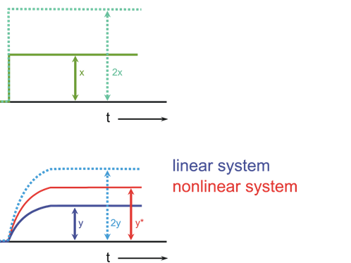
Fig. 1.5 Examples of step responses of (a) a linear and (b) a nonlinear system. x (t) input function, y (t) output function
The first task of a systems theory investigation is to determine the input-output relations of a system, in other words, to investigate the overall properties of the box in Figure 1.3 a. For this so-called "black box" analysis (or input-output analysis, or system identification) certain input values are fed into the system and then the corresponding output values are measured. For the sake of easier mathematical treatment, only a limited number of simple input functions is used. These input functions are described in more detail in Chapter 2 . In Figure 1.3b it is shown that the total system may be broken down into smaller subsystems, which are interconnected in a specific way. An investigation of the input-output relation of a system is thus followed immediately by the question as to the internal structure of the system. The second task of systems-theory research in the field of biology in thus to find out which subsystems form the total system and in what way these elements are interconnected. This corresponds to the step from Figure 1.3a to Figure 1.3b. In this way, we can try to reduce the system to a circuit which consists of a number of specifically connected basic elements. The most important of these basic elements will be explained in Chapter 4 .
For the black box analysis, the system is considered to be an element that transforms a known input signal into an unknown output signal. Taking this input-output relation as a starting point, attempts are made to draw conclusions as to how the system is constructed, i. e., what elements it consists of and how these are connected. (When investigating technical systems, usually the opposite approach is required. Here, the structure of the system is known and it is intended to determine, without experiments, the output values which follow certain input values that have not yet been investigated. However, such a situation can also occur in biology. For example, a number of local mechanisms of an ecosystem might have been investigated. Then the question arises to what extent the properties of the complete system could be explained?)
If the total system has been described at this level, we have obtained a quantitative model of a real system and the black box analysis is concluded. The next step of the investigation (i. e., relating the individual elements of the model to individual parts of the real system) is no longer a task of systems theory and depends substantially on knowledge of the system concerned. However, the model developed is not only a description of the properties of the overall system, but also is appropriate to guide further investigation of the internal structure of the system.
The first task of the systems theory approach is to describe the input-output properties of the system, such that its response to any input function can be predicted. The next step is to provide conclusions with respect to the internal structure of the system.
As was mentioned before, there are only a few functions usually used as input functions for investigating a system. Five such input functions will be discussed below. The investigation of linear systems by means of each of these input functions yields, in principle, identical information about the system. This means that we might just as well confine ourselves to studying only one of these functions. For practical reasons, however, one or the other of the input functions may be preferred in individual cases. Furthermore, and more importantly, this fundamental identity no longer applies to nonlinear systems. Therefore, the investigation of nonlinear systems usually requires the application of more than one input function.
Figure 2.1 a shows a step function. Here, the input value-starting from a certain value (usually zero)-is suddenly increased by a constant value at time t = t0 and then kept there. In theoretical considerations, the step amplitude usually has the value 1; therefore this function is also described as unit step, abbreviated to x(t) = 1(t). The corresponding output function (the form of which depends on the type of system and which therefore represents a description of the properties of the system) is called accordingly step response h(t) or the transient function.
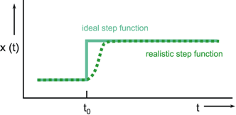
Fig. 2.1 The step function. Ideal (continuous line) and realistic version (dashed line)
The problem with using a step function is that the vertical slope can be determined only approximately in the case of a real system. In fact, it will only be possible to generate a "soft" trapezoidal input function, such as indicated in Figure 2.1 b. As a rule, the step is considered to be sufficiently steep if the rising movement of the step has finished before an effect of the input function can be observed at the output. This step function is, for example, particularly suitable for those systems where input values are given through light stimuli, since light intensity can be varied very quickly. In other cases, a fast change in the input function may risk damaging the system. This could be the case where, for example, the input functions are to be given in the form of mechanical stimuli. In this situation, different input functions should be preferred.
The response to a step function is called step response or transient function h(t).
As an alternative to the step function, the so-called impulse function x(t) = δ(t) is also used as input function. The impulse function consists of a brief pulse, i. e., at the time t = t0 the input value rises to a high value A for a short time (impulse duration Δt) and then immediately drops back to its original value. This function is also called Dirac, needle, δ, or pulse function. Mathematically, it can be defined as A Δt = 1, where Δt approximates zero, and thus A is growing infinitely. Figure 2.2 gives two examples of possible forms of the impulse function.
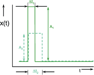
Fig. 2.2 Two examples of approximations of the impulse function. A impulse amplitude, Δt impulse duration
It is technically impossible to produce an exact impulse function. Even a suitable approximation would, in general, have the detrimental effect that, due to very high input values, the range of linearity of any system will eventually be exceeded. For this reason, usually only rough approximations to the exact impulse function are possible.
As far as practical application is concerned, properties of the impulse function correspond to those of the step function. Apart from the exceptions just mentioned, the impulse function can thus be used in all cases where the step function, too, could prove advantageous. This, again, applies particularly to photo reactions, since flashes can be generated very easily.
The response function to the impulse function is called impulse response or weighting function g(t). (In some publications, the symbols h(t) and g(t) are used in just the other way.) The importance of the weighting function in systems theory is that it is a means of describing a linear system completely and simply. If the weighting function g(t) is known, it will be possible to calculate the output function y(t) of the investigated system in relation to any input function x(t). This calculation is based on the following formula: (This is not to be proved here; only arguments that can be understood easily are given.)
y(t) = 0∫t g(t-t') x(t') dt'
This integral is termed a convolution integral, with the kernel (or the weighting function) g(t).
Figure 2.3 illustrates the meaning of this convolution integral. First, Figure 2.3a shows the assumed weighting function g(t') of an arbitrary system. By means of this convolution integral the intent is to calculate the response y(t) of the system to an arbitrary input function x(t') (Fig. 2.3b). (t and t' have the same time axis, which is shown with different symbols in order to distinguish between time t and the integration variable t'.)
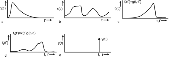
Fig. 2.3 The calculation of the convolution integral. (a) The weighting function g(t) of the system. (b) An arbitrary input function x(t'). (c) The signal of the weighting function g(t') is changed to g(-t') and it is shifted by t1, leading to f1 = g(t1 - t'). (d) The product f2(t') of the input function x(t') and g(t1 - t'). (e) The integral y(t) of this function f2(t') at time t1
To begin with, just the value of the output function y(t1) at a specific point in time t1 will be calculated. As the weighting function quickly approaches zero level, those parts of the input function that took place some time earlier exert only a minor influence; those parts of the input function that occurred immediately before the point in time t1 still exert a stronger influence on the value of the output function. This fact is taken into account as follows: The weighting function g(t') is reflected at the vertical axis, g(-t'), and then shifted to the right by the value t1, to obtain g(t1-t'), which is shown in Figure 2.3c. This function is multiplied point for point by the input function x(t'). The result f2(t') = x(t')g(t1 - t') is shown in Figure 2.3d. Thus, the effect of individual parts of the input function x(t') on the value of the output function at the time t, has been calculated. The total effect is obtained by summation of the individual effects. For this, the function f2(t') is integrated from 0 to t1, i. e., the value of the area below the function of Figure 2.3d is calculated. This results in the value y(t1) of the output function at the point in time t1 (Fig. 2.3e).
This process should be carried out for any t, in order to calculate point for point the output function y(t). If the convolution integral can be solved directly, however, the output function y(t) can be presented in a unified form.
The relation between weighting function (impulse response), g(t), and step response h(t) is as follows: g(t) = dh(t)/dt; h(t) = 0∫t g(t') dt'. Thus, if h(t) is known, we can calculate g(t) and vice versa. As outlined above, in the case of a linear system we can obtain identical information by using either the impulse function or the step function.
The response to an impulse function is called impulse response or weighting function g(t). Convolution of g(t) with any input function allows the corresponding output function to be determined.
In addition to the step and impulse functions, sine functions are quite frequently used as input functions. A sine function takes the form x(t) = a sin 2πν t (Fig. 2.4). a is the amplitude measured from the mean value of the function. ν (measured in Hertz = s-1) is the frequency of the oscillation. The expression 2πν is usually summarized in the so-called angular frequency ω: x(t) = a sin ω t. The duration of one period is 1/ν.
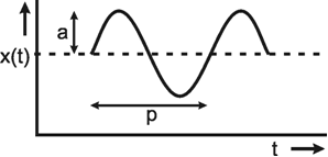
Fig. 2.4 The sine function. Amplitude a, period p = 1/ν. The mean value is shown by a dashed line
Compared to step and impulse functions, the disadvantages of using the sine function are as follows: in order to obtain, by means of sine functions, the same information about the system as if we were using the step response or impulse response, we would have to carry out a number of experiments instead of (in principle) one single one; i. e., we would have to study, one after the other, the responses to sine functions of constant amplitude but, at least in theory, to all frequencies between arbitrary low and infinitely high frequencies. In practice, however, the investigation is restricted to a limited frequency range which is of particular importance to the system. Nevertheless, this approach requires considerably more measurements than if we were to use the step or impulse function. Moreover, we have to pay attention to the fact that, after the start of a sinusoidal oscillation at the input, the output function, in general, will build up. The respective output function can be analyzed only after this build-up has subsided. The advantage of using sine functions is that the slope of the input function, at least within the range of frequencies of interest, is lower than that of step functions, which allows us to treat sensitive systems with more care.
The response function to a sine function at the input is termed frequency response. In a linear system, frequency responses are sine functions as well. They possess the same frequency as the input function; generally, however, they differ in amplitude and phase value relative to the input function. In this case, the frequency responses thus take the form y(t) = A sin (ω t + ϕ). The two values to be measured are therefore the phase shift ϕ between input and output function as well as change of the amplitude value. The latter is usually given as the ratio between the maximum value of the output amplitude A and that of the input amplitude a, i. e., the ratio A/a. Frequently, the value of the input amplitude a is standardized to 1, so that the value of the output amplitude A directly indicates the relation A/a. In the following this will be assumed in order to simplify the notation.
Both values, output amplitude A as well as phase shift ϕ, depend on the frequency. Therefore, both values are measured with a constant input amplitude (a = 1), but different angular frequencies ω. If the output amplitudes are plotted against the angular frequency ω, the result will be the amplitude frequency plot A(ω) of the system (Fig. 2.5a). Usually, both amplitude and frequency are plotted on a logarithmic scale. As illustrated in Figure 2.5a by way of a second ordinate, the logarithms of the amplitude are sometimes given. The amplitude frequency plot shown in Figure 2.5a shows that the output amplitude with a medium frequency is almost as large as the input amplitude, whereas it gets considerably smaller for lower and higher frequencies. Very often the ordinate values are referred to as amplification factors since they indicate the factor by which the size of the respective amplitude is enlarged or reduced relative to the input amplitude. Thus, the amplification factor depends on the frequency. (It is called dynamic amplification factor, as is explained in detail in Chapter 5 ).
An amplification factor is usually defined as a dimensionless value and, as a consequence, can only be determined if input and output values can be measured on the same dimension. Since this is hardly ever the case with biological systems, we have sometimes to deviate from this definition. One possibility is to give the amplification factor in the relative unit such as decibels (dB). For this purpose, one chooses an optional amplitude value A0 as a reference value (usually the maximum amplitude) and calculates the value 20 Ig (A1/A0) for every amplitude A1. A logarithmic unit in Fig. 2.5a thus corresponds to the value 20 dB. In Figure 2.5a (right ordinate) the amplitude A0 = 1 takes the value 0 dB.
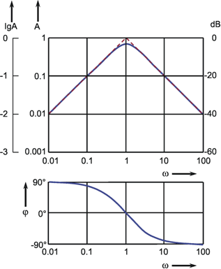
Fig. 2.5 The Bode plot consisting of the amplitude frequency plot (a) and the phase frequency plot (b). A amplitude, ϕ phase, ω = 2πν angular frequency. In (a) the ordinate is given as Ig A (far left), as A (left), and as dB (decibel, right)
In order to obtain complete information about the system to be investigated, we also have to determine changes in the phase shift between the sine function at the input and that at the output. By plotting the phase angle in a linear way versus the logarithm of the angular frequency, we get the phase frequency plot ϕ(ω) (Fig. 2.5b). A negative phase shift means that the oscillation at the output lags behind that of the input. (Due to the periodicity, however, a lag in phase by 270° is identical with an advance in phase by 90°). The phase frequency plot in Figure 2.5b thus means that in cases of low frequencies the output is in advance of the input by 90°, with medium frequencies it is more or less in phase, whereas at high frequencies it is lagging by about 90°.
Both descriptions, amplitude frequency plot and phase frequency plot, are subsumed under the term Bode plot. The significance of the Bode plot is dealt with in detail in Chapters 3 and 4 . We shall now briefly touch on the relationship between Bode plot and weighting function of a system. By means of a known weighting function g(t) of a system, it is possible to calculate, by application of the convolution integral, the sine response using the method explained in Chapter 2.2 :
y(t) = o∫t g(t-t') sin ω t' dt'.
The solution will be:
y(t) = A(ω) sin(ω t + ϕ(ω))
where A(ω) is the amplitude frequency plot and ϕ (ω) the phase frequency plot of the system (for proof, see e. g., Varju 1977 ). Thus, the sine function as an input function also gives us the same information about the system to be investigated as the step function or the impulse function.
As an alternative to the Bode plot, amplitude and phase frequency can be indicated in the form of the Nyquist or polar plot (Fig. 2.6). Here, the amplitude A is given by the length of the pointer, the phase angle is given by the angle between the x-axis and pointer. The angular frequency ω is the parameter, i.e., ω passes through all values from zero to infinity from the beginning to the end of the graph. In the example given in Figure 2.6, the amplitude decreases slightly at first in the case of lower frequencies; with higher frequencies, however, it decreases very rapidly. At the same time, we observe a minor lag in phase of output oscillation as compared to input oscillation if we deal with lower frequencies. This lag is increases to a limit of -180°, however, if we move to high frequencies.
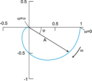
Fig. 2.6 The polar plot. A amplitude, ϕ phase, ω = 2πν angular frequency
The response to sine functions is called frequency response and is graphically illustrated in the form of a Bode plot or a polar plot.
An input function used less frequently is the statistical or noise function. It is characterized by the fact that individual function values follow one another statistically, i.e., they cannot be inferred from the previous course of the function. Figure 2.7 shows a schematic example. Investigating a system by means of a noise function has the advantage over using sine functions insofar as in principle, again, just one experiment is required to characterize the system completely. On the other hand, this can only be done with some mathematical work and can hardly be managed without a computer. (To do this, we mainly have to calculate the cross-correlation between input and output function. This is similar to a convolution between input and output function and provides the weighting function of the system investigated). Another advantage of the noise function over the sine function is that the system under view cannot predict the form of the input function. This is of particular importance to the study of biological systems, since here, even in simple cases, we cannot exclude the possibility that some kind of learning occurs during the experiment. Learning would mean, however, that the system has changed, since different output functions are obtained before and after learning on the same input function. By using the noise function, learning activities might be prevented. Changes of the property of the system caused by fatigue (another possible problem when investigating the frequency response) generally do not occur, due to the short duration of the experiment. The statistical function is particularly suitable for the investigation of nonlinear systems because appropriate evaluation allows nonlinear properties of the system to be judged ( Marmarelis and Marmarelis 1978 ).
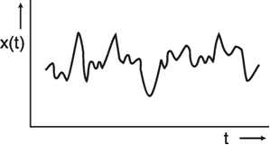
Fig. 2.7 An example of the statistical function
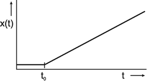
Fig. 2.8 The ramp function x(t) = kt (for t > t0)
Application of the statistical function is technically more difficult, both in experimental and in theoretical terms, but permits treatment of some properties of nonlinear systems.
The last of the input functions described here is the ramp function x(t) = kt. The ramp function has a constant value, e. g., zero, for t ≤ -t0 and keeps rising with a constant slope k for t > t0 (Fig. 2.8). Whereas the sine response requires us to wait for the building-up process to end before we can start the actual measurement, the very opposite is true here. As will be explained later ( Chapter 4 ), interesting information can be gathered from the first part of the ramp response. This also holds for the step and impulse functions. However, a disadvantage of the ramp function is the following. Since the range of possible values of the input function is normally limited, the ramp function cannot increase arbitrarily. This means that the ramp function may have to be interrupted before the output function (the ramp response) has given us enough information. In this case, a ramp-and-hold function is used. This means that the ramp is stopped from rising any further after a certain input amplitude has been reached and this value is maintained.
The advantage of the ramp function lies in the fact that it is a means of studying, in particular, those systems that cannot withstand the strong increase of input values necessary for the step function and the impulse function. A further advantage is that it can be realized relatively easily from the technical point of view.
For the investigation of nonlinear systems, ramp function and step function (contrary to sine function and impulse function) have the advantage that the input value moves in one direction only. If we have a system in which the output value is controlled by two antagonists, we might be able to study both antagonistic branches separately by means of an increasing and (through a further experiment) a decreasing ramp (or step) function. In biology, systems composed of antagonistic subsystems occur quite frequently. Examples are the control of the position of a joint by means of two antagonistic muscles or the control of blood sugar level through the hormones adrenaline and insulin. At the input side, too, there may be antagonistic subsystems such as, for example, the warm receptors that measure skin temperature, and which cause the frequency of action potentials to increase with a rise in temperature, and the cold receptors, causing the frequency of action potentials to decrease with a lower outside temperature.
The ramp function is easy to produce but might have difficulties experimentally because of the limited range of input values.
We cannot deal with the characteristics of simple elements in the next chapter until we have explained the significance of the Bode plot in more detail. For this reason we introduce here the concept of Fourier analysis. Apart from a number of exceptions that are of interest to mathematicians only, any periodic function y = f(t) may be described through the sum of sine (or cosine) functions of different amplitude, frequency and phase:

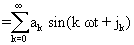
This is called a frequency representation of the function y(t) or the decomposition of the function to individual frequencies. The amplitude factors of the different components (ak) are called Fourier coefficients.
The concept of the Fourier decomposition can be demonstrated by the example of a square function (Fig. 3.1, yS). The Fourier analysis of this square function yields:
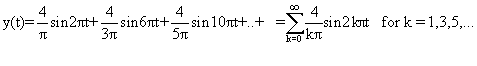
Frequency components that have an even numbered index thus disappear in this particular case. The first three components and their sum (y') have also been included in Figure 3.1.
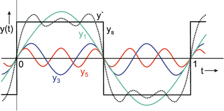
Fig.3.1 Fourier decomposition of a square function ys. The fundamental y1 = 3/π sin 2πt, and the two harmonics y3 = 4/(3π) sin 6πt and y5 = 4/(5π) sin 10πt are shown together with the sum y’ = y1 + y3 + y5 (dotted line).
As we can see, a rough approximation to the square function has already been achieved by y'. As this figure shows, in particular for a good approximation of the edges, parts of even higher frequency are required. The component with the lowest frequency (y1 in Fig. 3.1) is called the fundamental, and any higher-frequency parts are referred to as harmonic components. In these terms we might say that the production of sharp edges requires high-frequency harmonic waves.
This concept permits an easy qualitative interpretation of a given amplitude frequency plot. As can be seen from its amplitude frequency plot shown in Figure 3.2a, a system which transmits low frequencies well and suppresses high frequency components affects the transmission of a square function insofar as, in qualitative terms, the sharp edges of this function are rounded off. As Figure 3.1 shows, high-frequency components are required for a precise transmission of the edges. If the amplitude frequency plot of the system looks like that shown in Figure 3.2b, i. e., low frequencies are suppressed by the system whereas high frequency components are transmitted well, we can get a qualitative impression of the response to a square wave in the following way. Providing we subtract the fundamental wave y1 from the square function ys which would occur where all frequencies are transmitted equally well, it would turn out that there would be a good transmission within the range of the edges and a poor transmission within the range of the constant function values, if the lower frequencies were suppressed. As a result, the edges would be emphasized particularly strongly.
Due to the fact that, in most systems (see, however, Chapter 10 ), different frequency components undergo different phase shifts which we have not discussed so far, these considerations are only of a qualitative nature. The quantitative transfer properties of some systems will be dealt with in Chapter 4 . It can already be seen, however, that the amplitude frequency plot allows us to make important qualitative statements concerning the properties of the system.
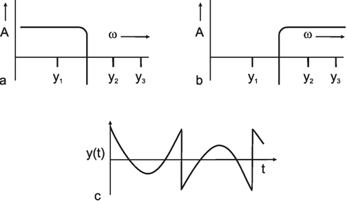
Fig. 3.2 Assume a system having a negligible phase shift and showing an amplitude frequency plot which transmits low frequencies like that of the fundamental y1 in Fig. 3.1 but suppresses higher frequencies like y3 or y5. A square wave as shown in Fig. 3.1 given at the input of this system would result in an output corresponding to the sine wave of y1. When the system is assumed to have a mirror-image-like amplitude frequency plot, (b), the response to the square wave input would look like the square wave without its fundamental. This is shown in (c)
We are now able to realize more clearly why investigation of a linear system by means of step or impulse functions requires, in principle, only one experiment to enable us to describe the system, whereas in the case of an investigation by means of sine functions we need to carry out, theoretically, an infinite number of experiments. The reason is that the edges of step and impulse functions already contain all frequency components. These have to be studied separately, one after another, if we use sine functions.
The Fourier analysis shows that sharp edges of a function are represented by high frequency components and that low frequencies are necessary to represent the flat, horizontal parts of the function.
So far we have only considered how to obtain information about the transfer properties and thus to describe the system to be investigated; now we have a further task: how to determine the internal structure of the system from the form of the Bode plot or the weighting function. This is done in the following way: we try to break down the total system into elements, called filters. Below we describe the properties of the most important filters. Subsequently, using an example based on the transfer properties of a real system, we will show how to obtain the structure of the system by suitably composing elementary filters.
A low-pass filter allows only low frequencies to pass. As can be seen in the amplitude frequency plot of the Bode plot (Fig. 4.1a), low frequency sine waves are transmitted by the amplification factor 1; high frequency sine waves, however, are suppressed. The graph of the amplitude-frequency plot may be approximated by means of two asymptotes. One of those runs horizontally and in Figure 4.1 a corresponds to the abscissa. The second asymptote has a negative slope and is shown as a dashed line in Figure 4.1 a. If the coordinate scales are given in logarithmic units, this line has the slope -1. The intersection of both asymptotes marks the value of the corner frequency ω0, also called the characteristic frequency. At this frequency, the output amplitude drops to about 71 % of the maximum value reached with low frequencies. In the description chosen here, ω0 is set to 1. By multiplying the abscissa values with a constant factor, this Bode plot can be changed into that of a low-pass filter of any other corner frequency.
As the phase-frequency plot shows, there is practically no phase shift with very low frequencies; the phase-frequency plot approaches zero asymptotically. With very high frequencies, there is a lag in phase of the output oscillation, compared to the input oscillation, by a maximum of 90°. In the case of the corner frequency ω0 ( = 2πν0) the phase shift comes to just 45°.
Besides the sine function, the other important input function is given by the step function. The transient, or step response h(t) of this low-pass filter is shown in Figure 4.1 b. It starts at t = 0 with a slope of 1/τ and asymptotically approaches horizontal. The amplitude value of this line indicates the static amplification factor of the system, which has been assumed to be 1 in this example. This static amplification factor corresponds to the amplification factor for low frequencies which can be read off from the amplitude-frequency plot. The time constant τ of this low-pass filter can be read from the step response to be the time at which the response has reached 63% of the ultimate value, measured from time t = 0.The transition phase of the function is also referred to as the dynamic part and the plateau area as the static part of the response (see also Chapter 5 ). For a decreasing step, we obtain an exponential function with negative slope.
Here, the time constant indicates the time within which the exponential function e-1/τ from an amplitude value A has dropped to the amplitude value A/e, i. e., to about 37 % of the value A.
Corner frequency ω0 and time constant τ of this low-pass filter (and of the corresponding high-pass filter, which will be described in Chapter 4.2 ) are related in the following way:
 .
.
Thus, the time constant of this low-pass filter can also be obtained from the Bode plot, to be τ = 1 s. (In the case of the Bode plot, and in all of the following figures in Chapter 4 , the response functions of filters for other corner frequencies and time constants can be obtained by expansion of the abscissa by an appropriate factor). The formula for the impulse response shown in Figure 4.1 b is only applicable for the range t > 0. For the sake of simplicity, this restriction will not be mentioned further in the corresponding cases that follow.
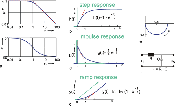
Fig. 4.1 Low-pass-filter. (a) Bode plot consisting of the amplitude frequency plot (above) and the phase frequency plot (below). Asymptotes are shown by red dashed lines. A amplitude, ϕ phase, ω = 2πν angular frequency, (b) step response, (c) impulse response, (d) ramp response. In (b)-(d) the input functions are shown by green lines. The formulas given hold for t > 0. k describes the slope of the ramp function x(t) = kt. (e) polar plot. (f) Electronic wiring diagram, R resistor, C capacitor, τ time constant, u1 input voltage, u0 output voltage
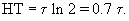
The easiest way to check whether a given function is an exponential one is to plot it on a semilogarithmic scale (with logarithmic ordinate and linear abscissa). This will result in a line with the slope -1/τ. Quite often the half-time or half-life is used as a measure of duration of the dynamic part instead of the time constant τ. It indicates the time by which the function has reached half of the static value. Given a filter of the first order (also true for the corresponding high-pass filter, see Chapter 4.2 ) the relation between halftime (HT) and time constant is as follows:
Because of the step response, a low-pass filter may be understood intuitively to be an element which though it tries to follow the input value proportionally, succeeds only after a temporal lag due to some internal sluggishness. Figure 4.2 shows an example of low-pass-like behavior. Here, the force produced by a muscle is shown when the frequency of action potentials within the relevant motoneuron has been changed.
The impulse response, i. e., the weighting function g(t) of this low-pass filter, is shown in Figure 4.1 c. If the input value zero has been constant for a long time, the output value is, at first, also zero. During the application of the impulse function at time t = 0 however, the output jumps to the value 1/ τ and then, starting with the slope -1/ τ2 decreases exponentially, with the time constant τ, to zero. The maximum amplitude 1/τ can be reached only if an ideal impulse function is used, however.
The weighting function of this lowpass filter is described by:
 .
.
Figure 4.1 d shows the ramp response of a low-pass filter. It starts with a horizontal slope at the beginning of the ramp and asymptotically approaches a straight line that is parallel to the input function x(t) = kt. This line intersects the time axis at the value τ. For the sake of completeness, the Nyquist plot has also been given in Figure 4.1e. However, this will not be described in more detail here or in further examples, since it contains the same information given in the Bode plot, as we have already mentioned above.
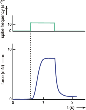
Fig. 4.2 The response of an insect muscle to an increasing and a decreasing step function. The input function (upper trace) is given by the experimentally induced spike frequency of the motorneuron. The output function (lower trace) shows the force developed by the muscle (after Iles and Pearson 1971 )
Systems that possess low-pass characteristics can be found everywhere, since - for physical reasons - there is no system that is able to transmit frequencies with no upper limit. In order to investigate the properties of such a filter, it is most convenient to construct it of electronic components. The simplest electronic low-pass filter is shown in the wiring diagram in Figure 4.1 f. It consists of an ohmic resistor R and a capacitor C. The input function x(t), given as voltage, is clamped at ui, the output function y(t) is measured as voltage at u0. The time constant of this low-pass filter is calculated by τ = RC. Electronic circuits of this kind are also indicated accordingly for systems discussed later. Alternatively, a low-pass filter can be simulated on a digital computer as described in Appendix II .
A low-pass filter describes a system with sluggishness, i. e., one in which high frequency components are suppressed. Dynamic properties are described by the time constant τ or the corner frequency ω0.
A high-pass filter permits only high frequencies to pass, while suppressing the low frequency parts. This is shown by the amplitude frequency, plot in Fig. 4.3a, which is the mirror image of tat of the low-pass filter (Fig. 4.1). When logarithmic coordinates are used, the asymptote along the descending branch of the amplitude frequency plot takes the slope + 1. As with the low pass filter, the corner frequency is indicated by the intersection of the two asymptotes. Similarly, the time constant is calculated according to τ = 1/ω0. Here though, the corner frequency indicates that those oscillations are permitted to pass whose frequencies are higher than the corner frequency, while oscillations whose frequencies are markedly lower than the corner frequency, are suppressed.
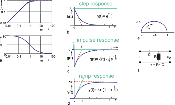
Fig. 4.3 High-pass filter. (a) Bode plot consisting of the amplitude frequency plot (above) and the phase frequency plot (below). Asymptotes are shown by red dashed. A amplitude, ϕ phase, ω = 2πν angular frequency. (b) step response, (c) impulse response, (d) ramp response. In (b) - (d) the input functions are shown by green lines. The formulas given hold for t > 0. k describes the slope of the ramp function x(t) = kt. (e) polar plot. (f) Electronic wiring diagram, R resistor, C capacitor, τ time constant, u1 input voltage, uo output voltage
As with the low-pass filter shown in Figure 4.1, the corner frequency is assumed to be ω0 = 1 s-1 and the time constant to be τ = 1 s. When examining the phase-frequency plot, we notice a phase lead of output oscillation compared to input oscillation by maximally + 90° for low frequencies. For the corner frequency it amounts to +45°, asymptotically returning to zero value for high frequencies.
The step response (Fig. 4.3b) clearly illustrates the qualitative properties of a high-pass filter. With the beginning of the step, the step response instantly increases to the value 1, and then, with the initial slope -1 /τ and the time constant τ, decreases exponentially to zero, although the input function continues to exhibit a constant value of 1. The maximum amplitude takes value 1 since, as can be gathered from the location of the horizontal asymptote of the amplitude-frequency plot, the amplification factor of this high-pass filter is assumed to be 1. The amplification factor in the static part of the step response (static amplification factor) is always zero. By contrast, the value to be taken from the horizontal asymptote of the amplitude-frequency plot is called maximum dynamic amplification factor kd. (See also Chapter 5 ).
As in the case of the low-pass filter, the impulse response is represented in Figure 4.3c by assuming a mathematically ideal impulse as input. The response also consists of an impulse that does not return to value zero, however, but overshoots to -1/τ, and then, with the time constant τ, exponentially returns to zero. The impulse response thus consists of the impulse function δ(t) and the exponential function -(1/τ)e-t/τ. With an impulse function of finite duration, the duration of the impulse response and the amplitude of the negative part increase accordingly. (For details, see Varju 1977 ).
Whereas intuitively one could call a low-pass filter an inert element, a high-pass filter constitutes an element that merely responds to changes, but not to permanently constant values at the input. Such properties are encountered in sensory physiology, in the so-called tonic sensory cells, which respond in a low-pass manner, and in the so-called phasic sensory cells, which respond in a high-pass manner. The step response of such high-pass-like sensory cells is shown in Figure 4.4.
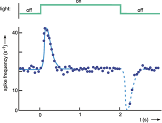
Fig. 4.4 The response of a single fiber of the optical nerve of Limulus. As input function light is switched of for 2 seconds (upper trace). The output function shows the instantaneous spike frequency (each dot is calculated as 1/Δt, Δt being the time difference between two consecutive spikes). The solid blue line shows an approximation of the data. The dashed part (response to the decreasing step) represents the mirror image of the first part of the approximation (after Ratliff 1965 ). Note that negative spike frequencies are not possible
This behavior in biological systems is frequently called adaptation. In mathematical terms, one could speak of a differentiating behavior since, especially with very short time constants, the first derivative of the input function is formed approximately by a high-pass filter.
The ramp response of this high-pass filter is shown in Figure 4.3 d. It starts at t = 0 and a slope k, the slope of the input function, and then, with the time constant τ, increases to the plateau value k τ. In order to obtain the time constant of the high-pass filter from the ramp response, the range of values available for the input function has to be sufficiently great such that the plateau at the output can be reached while the ramp is increasing. Conversely, with the given input range A, the slope k of the ramp has to be correspondingly small. If it is assumed that the plateau is reached approximately after the triple time constant, then k ≤ A/3τ.
Like those for the low-pass filter, Figure 4.3e illustrates the polar plot of the high-pass filter and Figure 4.3f an electronic circuit. This circuit also consists of an ohmic resistor R and a capacitor C, but in reverse order this time. The time constant is also calculated as τ = R C. For a digital simulation see Appendix II .
A high-pass filter describes a system which is only sensitive to changes in the input function. It suppresses the low frequency components, which qualitatively corresponds to a mathematical differentiation. The dynamic properties are described by the time constant r or the corner frequency ω0.
If n low-pass filters are connected in series, a low-pass of the n-th order is obtained. If two systems with specific amplification factors are connected in series, we obtain the amplification factor of the total system by multiplying the two individual amplification factors. As mentioned in Chapter 3 , the amplitude-frequency plot of a system reflects the amplification factors valid for the various frequencies. In order to obtain the amplitude-frequency plot of a 2nd order filter, it is thus necessary to multiply the amplitude values of the various frequencies (or, which is the same, add up their logarithms). This is why the logarithmic ordinate is used in the amplitude-frequency plot in the Bode plot: the amplitude frequency plot of two serially connected filters can be obtained simply by adding the amplitude frequency plots of the two individual filters, point by point if logarithms are used, as shown in the right hand ordinate of Figure 4.5 a. (See also Figure 2.5).
In addition to the amplitude frequency plot of a 1st order low-pass filter (already shown in Figure 4.1) Figure 4.5a shows the amplitude frequency plots of low-pass filters of the 2nd, 3rd, and 4th order, which are obtained by serially-connecting several identical 1st order low-pass filters. The corner frequency remains the same, but the absolute values of the slope of the asymptote at the descending part grows proportionately steeper with the order of the filter. This means that the higher the order of the low-pass filter, the more strongly high frequencies are suppressed. (Systems are conceivable in which the slope of the descending part of the amplitude frequency plot shows values that lie between the discrete values presented here. The system would then not be of an integer order. In view of the mathematical treatment of such systems, however, the reader is referred to the literature. (See e.g., Varju 1977 ).
If a sine wave oscillation undergoes a phase shift in a filter, and if several filters are connected in series, the total phase shift is obtained by linear addition of individual phase shifts. Since the value of the phase shift depends on the frequency, the phase frequency plot of several serially connected filters is obtained directly by a point-by-point addition of individual phase-frequency plots. For this reason, the phase frequency plot in the Bode plot is shown with a linear ordinate. Figure 4.5a shows that, at low frequencies, phase shifts are always near zero but for higher frequencies, they increase with the increasing order of the low-pass filter.
In the step responses (Fig. 4.5b), the initial slope decreases with an increasing order, although the maximum value remains constant (presupposing the same static amplitude factor, of course). In the impulse responses shown in Figure 4.5c, both the initial slope, and the maximal amplitude of the impulse response, decrease with increasing order of the low-pass filter. Generation of the form of an impulse response or a step response of a filter of a higher (e. g., 2nd) order can be imagined as follows. The response of the first filter to the impulse (or step) function at the same time represents the input function for the second filter. This, in turn, qualitatively influences the new input function in a corresponding way. In the case of low-pass filters, output functions of the second low-pass filter will thus be much flatter.
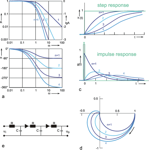
Fig. 4.5 Low-pass filter of nth order. (a) Bode plot, A amplitude, ϕ phase, ω angular frequency. (b) step response, (c) impulse response, (d) polar plot. n = 1 to 4 refers to the order of the filter. In (b) and (c) the input functions are shown by green lines. (e) Electronic wiring diagram for n = 3. The triangles represent amplifiers with gain 1, R resistor, C condensor, ui input voltage, uo output voltage
The formulas for impulse and step responses of low-pass filters of higher order are shown in the table in Appendix I . When a higher order filter is simulated by an electronic circuit, the individual filter circuits have to be connected via a high impedance amplifier to avoid recurrent effects. This is symbolized by a triangle in Figure 4.5e. Figure 4.5d contains the polar plots for low-pass filters of the 1st through the 4th order. The properties of low-pass filters which rely on recurrent effects are discussed in Chapter 4.9 .
The Bode plot of two serially connected filters is obtained by adding the logarithmic ordinate values of the amplitude frequency plot and by linear summation of the phase frequency plot. Low-pass filters of higher order show stronger suppression and greater phase shifts of high frequency components.
If n high-pass filters are serially connected, the result is called a n-th order high-pass filter. The Bode plot (Fig. 4.6a) and polar plot (Fig. 4.6c) will be mirror images of the corresponding curves of low-pass filters shown in Figure 4.5. Here, too, the value of the corner frequency remains unchanged, whereas the slope of the asymptote approaching the descending part of the amplitude frequency plot increases proportionate to the order of the high-pass filter. For very high frequencies, the phase frequency plots asymptotically approach zero. By contrast, for low frequencies, the phase lead is the greater, the higher the order of the high-pass filter.
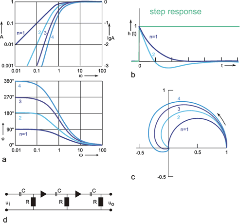
Fig. 4.6 High-pass filter of nth order. (a) Bode plot, A amplitude, ϕ phase, ω angular frequency. (b) step response, (c) polar plot. n = 1 to 4 refers to the order of the filter. In (b) the input function is shown by green lines. (b) Electronic wiring diagram for n = 3.The triangles represent amplifiers with gain 1, R resistor, C condensor, ui input voltage, uo output voltage
In addition to the step response of the 1st order high-pass filter (already shown in Figure 4.3 c) Figure 4.6b shows the step response of the 2nd order high-pass filter. After time T, this crosses the zero line and then asymptotically approaches the abscissa from below. The corresponding formula is given in the table in Appendix I . The origin of this step response can again be made clear intuitively by taking the step response of the first 1st order high-pass filter as an input function of a further 1st order high-pass filter. The positive slope at the beginning of this new input function results in a positive value at the output. Since the input function subsequently exhibits a negative slope, the output function will, after a certain time (depending on the value of the time constant), take negative values, eventually reaching zero, as the input function gradually turns into a constant value.
In a similar way, it can be imagined that the step response of a 3rd order high-pass filter, which is not shown here, crosses the zero line a second time and then asymptotically approaches the abscissa from the positive side. Figure 4.6d shows an electronic circuit with the properties of 3rd order high-pass filter as an example.
High-pass filters of higher order show stronger suppression and greater phase shifts of low-frequency components. Qualitatively, they can be regarded as to produce the nth derivative of the input function.
In practice, a pure high-pass filter does not occur since no system can transmit arbitrary high frequencies. Therefore, every real system endowed with high-pass properties also has an upper corner frequency, which is given by the ever-present low-pass properties. A "frequency band," which is limited on both sides, is thus transmitted in this case. We, therefore, speak of a band-pass filter. A band-pass filter is the result of a series connection of high- and low-pass filters. In linear systems, the serial order of both filters is irrelevant. Amplitude and phase frequency plots of a band-pass filter can be obtained by logarithmic or linear addition of the corresponding values of individual filters, as described in Chapter 4.3 .
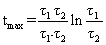
The Bode plot of a symmetrical band-pass filter (i. e., where the high- and low-pass filter are of the same order) is shown in Figure 4.7a. As can be seen from the slope of the asymptotes approaching the ascending and the descending parts of the amplitude frequency plot, the low-pass filter and the high-pass filter are both of 1st order. The corner frequency of the high-pass filter is 1 Hz, that of the low-pass filter 100 Hz in this example. Figure 4.7b, c show the step response and the impulse response of this system.
The amplitude frequency plot does not necessarily indicate the time constants or corner frequencies of each filter. As described in Chapter 4.1 and 4.2 , the values of the corner frequencies can be read from the intersection of the horizontal asymptote and the ascending asymptote (high-pass filter) or the descending asymptote (low-pass filter). A horizontal asymptote can only be plotted, however, if the corner frequency of the low-pass filter is sufficiently high compared to that of the high-pass filter, such that the amplitude frequency plot exhibits a sufficiently long, horizontal part. But if both corner frequencies are too similar, as in the example shown in Figure 2.5, or if the corner frequency of the low-pass filter is even lower than that of the high-pass filter, no statement is possible concerning the position of the horizontal asymptote on the basis of the amplitude frequency plot. (It should be stressed here that the amplification factor need not always be 1, although this has been assumed in examples used here, for the sake of clarity). In the band-pass filter shown in Figure 2.5, the upper and lower corner frequencies are identical in this particular case. As an illustration, the corresponding step response and the impulse response of this system are shown in Figure 4.7d, e.
Contrary to the Bode plot, the step and the impulse responses of two serially connected filters cannot be computed as easily from the step or impulse responses of each filter. The corresponding formulas for this case, as for the general case of different time constants, are given in Appendix I . For computation of the step and impulse responses of symmetrical or asymmetrical bandpass filters of a higher order, the reader is also referred to Appendix l. For the case of a symmetrical 1st order band-pass filter of different time constants, i. e., τ1 (low-pass filter) ≠ τ2 (high-pass filter), the time when the step response reaches its maximum is given by
 .
.
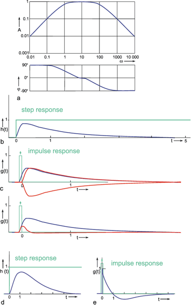
Fig. 4.7 Band-pass filter consisting of serially connected 1st order low-pass and high-pass filters. (a) Bode plot, A amplitude, ϕ phase, ω angular frequency, lower corner frequency (describing the high-pass properties): 1 Hz, upper corner frequency (describing the low-pass properties): 100 Hz. (b) Step response. (c) Impulse response. (d) and (e) Step and impulse responses of a band-pass filter whose upper and lower corner frequencies are identical (1 Hz). The Bode plot of this system is given in Fig. 2.5. In (b) to (e) the input functions are shown by green lines
A band-pass filter can be considered as serial connection of low-pass and high-pass filters. Its dynamics can be described by a lower and an upper corner frequency, marking a "frequency band.”
In the above section we have treated the basic types of filters and have shown how to connect them in series. Alternatively, filters might be connected in parallel. To discuss a simple example, we connect a low-pass filter and a high-pass filter with the same time constant in parallel. If the branch with the high-pass filter is endowed with an amplification k, and the outputs of both branches are added (Fig. 4.8a), we obtain different systems depending on the factor k. For the trivial case k = 0 the system corresponds to a simple low-pass filter.
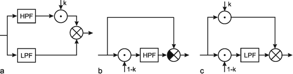
Fig. 4.8 Three diagrams showing the same dynamic input-output behavior. (a) A parallel connection of a high-pass filter (HPF) and a low-pass filter (LPF). The high-pass branch is endowed with a variable gain factor k. (b) The corresponding system containing only a high-pass filter, and (c) only a low-pass filter
If k takes a value between 0 and 1, we obtain a lag-lead system. As we have seen in the series connection of two filters, the Bode plot of the total system can be computed from the individual Bode plots by simple addition, while the computation of the step response is more difficult (see Chapter 4.3 , 4.5 ). The opposite is true for parallel connection. Here, the step response of the total system can be computed by means of a point-by-point addition of the step responses of the two individual branches. Figure 4.9 b indicates the step responses of the two branches for the case k = 0.5 by dotted lines, and the sum of both functions, i. e., the step response of the total system, by a bold line. At the start of the input step, this function thus initially jumps to value k, and then, with the initial slope (1 - k)/τ and the time constant τ, asymptotically approaches the final value 1.
If the amplitude frequency plot of the total system is to be determined from that of each of the two branches, the correct result certainly will not be achieved by a point-by-point multiplication (logarithmic addition), as is possible in series connected filters. Nor does a linear addition produce the correct amplitude frequency plot of the total system. Since the oscillations at the output, responding to a particular sine function at the input, generally experience a different phase shift in each branch, (i. e., since their maxima are shifted relative to each other) a sine function is again obtained after addition. Because of this shift, the maximum amplitude of this function will normally be less than the sum of the maximum amplitudes of the two individual sine waves. In computation of the amplitude frequency plot of the total system, the corresponding phase shifts must, therefore, be taken into account.
For the same reasons, the phase frequency plot cannot be computed in a simple manner, either. However, a rough estimate is possible for specific ranges both of the amplitude and the phase frequency plots (Fig. 4.9a). Thus, for very low frequencies, the contribution of the high-pass filter is negligible. The amplitude and phase frequency plots of the total system will therefore approximate those of the low-pass filter. This means that the horizontal asymptote of the amplitude frequency plot is about 1, and that, starting from zero, the phase frequency plot tends to take increasingly negative values.
Conversely, for high frequencies, it is the contribution of the low-pass filter that is negligible. The amplitude and phase frequency plots of the total system thus approximate those of the high-pass filter, and the amplitude frequency plot is endowed, in this range, with a horizontal asymptote at the amplification factor of k = 0.5. The phase frequency plot again approaches zero value from below.
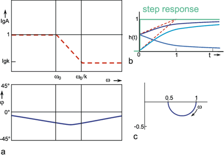
Fig. 4.9 The lag-lead system, i. e., a parallel connection of a low-pass filter and a high-pass filter with k < 1 (see Fig. 4.8a). (a) The amplitude frequency plot is only shown by the three assymptotes. (b) The step responses of the two branches for the case k = 0.5 are shown by light blue lines, and the sum of both functions, i. e. the step response of the total system, by a dark blue line. The input function is shown by green lines. (c) polar plot for k = 0.5
In the middle range, the phase frequency plot is located between that of the high-pass filter and that of the low-pass filter. In Figure 4.9a, the amplitude frequency plot is indicated only by its asymptotes (a widely used representation in the literature). The asymptote in the middle range exhibits the slope -1 on a logarithmic scale. The intersections of this asymptote with the two others occur at the frequencies w0 and w0/k. Its Nyquist plot is shown in Figure 4.9c.
If the value of k is greater than 1, we speak of a lead-lag system. The step response is again obtained by a point-by-point addition of the low-pass response as well as of the correspondingly amplified high-pass response, shown in Figure 4.10b by dotted lines. As in the previous case, it immediately jumps to value k at the beginning of the step, and then, with the initial slope (1-k)/τ and the time constant τ, decreases to the final value 1.
The amplitude frequency plot of the lead-lag system is indicated in Figure 4.10a only by its three asymptotes, as in the case of the lag-lead system. Since the value of k is greater than 1, the horizontal asymptote in the range of high frequencies appears here above the corresponding asymptote in the range of low frequencies. The two intersections of the three asymptotes again lie at the frequencies ω0 and ω0/k, whereas the asymptote approaching the middle range exhibits the slope + 1 on a logarithmic scale.
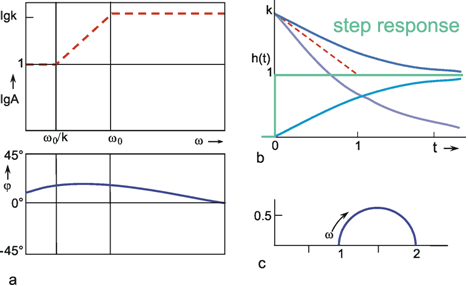
Fig. 4.10 The lead-lag system, i. e., a parallel connection of a low-pass filter and a high-pass filter with k > 1 (see Fig. 4.8 a). (a) The amplitude frequency plot is only shown by the three asymptotes. (b) The step responses of the two branches for the case k = 2 is shown by light blue lines, and the sum of both functions, i. e., the step response of the total system, by a dark blue line. The input function is shown by green lines. (c) polar plot for k = 2
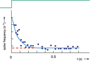
Fig. 4.11 Step response of a mammalian muscle spindle. When the muscle spindle is suddenly elongated (green line), the sensory fibers show a sharp increase in spike frequency which later drops to a new constant level which is, however, higher than it was before the step. Ordinate in relative units (after Milhorn 1966 )
In Chapter 3 , it was pointed out that an edge of a function is produced by high-frequency components. The large amplification factor in the high-frequency range that can be recognized in the amplitude frequency plot thus corresponds to the "over-representation" of the edge in the step response. On account of the larger amplification factor in the high-pass branch, the high-pass properties predominate to such an extent that the phase shift is positive for the entire frequency range. As can be expected in view of what has been discussed above, however, they asymptotically approach zero value, both for very high and very low frequencies. The corresponding Nyquist plot is shown in Figure 4.10c.
The behavior of a lead-lag system thus corresponds to that of the most widespread type of sensory cell, the so-called phasic-tonic sensory cell. Muscle spindles, for example, exhibit this type of step response (Fig. 4.11). (It should be noted, however, that there are also nonlinear elements which show similar behavior.)
If a lead-lag system is connected in series with a low-pass filter, the phasic part of the former can compensate for a considerable amount of the inert properties of the low-pass filter. This might be one reason for the abundancy of phasic-tonic sensory cells. (See also Chapter 8.6 ).
The system addressed here is described by the diagram shown in Figure 4.8a, but the same input-output relations are exhibited by the connection shown in Figure 4.8b. The origin of the responses of this system can be thought of as the high-pass response (which belongs to the input function and is multiplied by the factor 1-k), subtracted from the input function itself. The direct summation of the input onto the output dealt with here might be called "feed forward summation". The connection shown in Figure 4.8c also exhibits the same properties. Here, the input function, which is multiplied by the factor k, is added to the corresponding low-pass response, which is endowed with the factor (1-k).
To determine the transfer properties of filters connected in parallel, consideration of step responses is similar than for frequency responses. Lag-lead and lead-lag systems are simple examples of parallel connected high-pass and low-pass filters. The lead-lag system corresponds to the so-called phasic-tonic behavior of many neurons, in particular sensory cells.
Especially in biological systems, a pure time delay is frequently observed, in which all frequencies are transmitted without a change of amplitude and with merely a certain time delay or dead time T. The form of the input function thus remains unchanged. The entire input function is shifted to the right by the amount T, however. Such pure time delays occur whenever data are transmitted with finite speed. This occurs, for example, in the transmission of signals along nerve tracts, or transport of hormones in the bloodstream.
Since the amplitudes are not influenced by a pure time delay, the amplitude frequency plot obtained is a horizontal line at the level of the amplification factor (Fig: 4.12a). The phase shift, on the other hand, takes increasingly negative values with increasing frequency such that ϕ(ω) = -ω T. The reason for this is that, compared to the oscillation period which decreases at higher frequencies, the constant dead time increases in relative terms. The value of dead time can be read from the phase frequency plot as follows. It corresponds to the oscillation period ν = ω/2π, in which a phase shift of exactly - 2π or - 360° is present. The phase frequency plot of a pure time delay thus, unlike that of the other elements discussed so far, does not approximate a finite maximum value. Rather, the phase shifts increase infinitely for increasing frequencies. The corresponding Nyquist plot is shown in Figure 4.12c. (Confusion may be caused by the fact that, in some textbooks, the oscillation period T = 1/ν, the dead time (in this text), as well as the time constant, may be referred to by the letter T.)
An electronic system endowed with the properties of a pure dead time requires quite a complicated circuit. However, it can be simulated very simply using a digital computer. (See Appendix II ).
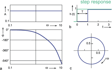
Fig. 4.12 Pure time delay. (a) Bode plot, A amplitude, ϕ phase, ω = 2πν angular frequency. (b) step response, the input function is shown by green lines, T dead time. (c) polar plot
A pure time delay or dead time unit does not influence the amplitudes of the frequency components but changes the phase values the more the higher the frequency.
An Asymmetrical Band-Pass Filter
In the following experiment a visual reflex of an insect is investigated. A locust is held by the thorax and a pattern, consisting of vertical black and white stripes, is moved sinusoidally in horizontal direction in front of it ( Thorson 1966 ). According to the well-known optomotor response, the animal tries to follow the movement of the pattern by moving its head correspondingly. However, the head is fixed to a force transducer and the forces are measured by which it tries to move its head using its neck muscles. The amplitude and the phase shift of the sinusoidally varying forces are measured in dB (Fig. B1.1). How could this result be interpreted in terms of filter theory? Regarding the amplitude frequency plot, the slope of the asymptote for high frequency values (i. e., > 0.5 Hz) is approximately -1, indicating a 1st order low-pass filter. Note that 20 d8 correspond to one decade ( Chapter 2.3 ). The asymptote to the low frequency values is approximately 0.5 and thus has to be interpreted as a high-pass filter of 0.5th order. Thus, as a first interpretation we could describe the system as a serial connection of a 1st order low-pass filter and a 0.5th order high-pass filter. Does the phase frequency plot correspond to this assumption? A high-pass filter of 0.5th order should produce a maximum phase shift of 45° for low frequencies, as was actually found. For high frequencies, a 1 st order low-pass filter should lead to a maximum phase shift of -90°. However, a somewhat larger phase shift is ob served. Thus, the results could only be described approximately by a band-pass filter which consists of a 1st order low-pass filter and a 0.5th order high-pass filter. The larger phase shifts could be caused by a pure time delay. The step response revealed a dead time of 40 ms. For the frequency of 1 Hz this leads to an additional phase shift of about 15° and for 2 Hz to a phase shift of about 30°. The phase shifts produced by such a pure time delay for the three highest frequencies used in the experiment are shown by open circles. These shifts correspond approximately to the differences between the experimental results and the values expected for the band-pass filter. Thus, the Bode plot of the system can reasonably be described by an asymmetrical band-pass filter and a pure time delay connected in series.
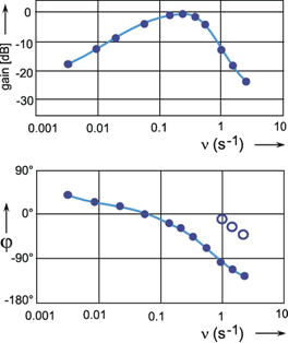
Fig. B 1.1 Bode plot of the forces developed by the neck muscles of a locust. Input is the position of a sinusoidally moved visual pattern. ν is stimulus frequency. The gain is measured in dB (after Thorson 1966 )
Whenever integration is carried out in a system (e. g., if, in a mechanical system, force (or acceleration) is to be translated into speed, or the latter is to be translated into position) such a process is described mathematically by an integrator. Within the nervous system, too, integration is performed. For example in the case of the semicircular canals, integrators have to ensure that the angular acceleration actually recorded by these sense organs, is transformed somewhere in the central nervous system into the angular velocity perceived by the subject.
The step response of an integrator is a line ascending along a slope τi from the beginning of the step (Fig. 4.13b). τi is called the integration time constant. It denotes the time that elapses before the response to a unit step reaches value 1. The "amplification factor" of an integrator is thus inversely proportional to τi (k = 1/τi) and hence takes the dimension s-1. In accordance with the properties of an integrator, the impulse response jumps to value 1 and remains there (Fig. 4.13c). The amplitude frequency plot of an integrator consists of a line descending along a slope -1 in the logarithmic plot. This means that the lower the input frequency, the more the amplitudes are increased, and that high frequency oscillations are considerably damped. The amplitude frequency plot crosses the line for the amplification value 1 at ω = 1/τi. For all frequencies, the phase shift is a constant -90°. Figure 4.13d shows the symbol normally used for an integrator.
An integrator might also be described by a system, the output of which does not solely depend on the actual input but also on its earlier state. This requires the capability of storing the earlier value. Therefore an integrator can also be represented by a unit with recurrent summation (Fig. 4.13e). This permits an easy way of implementing an integrator in a digital computer program (see Appendix II ).
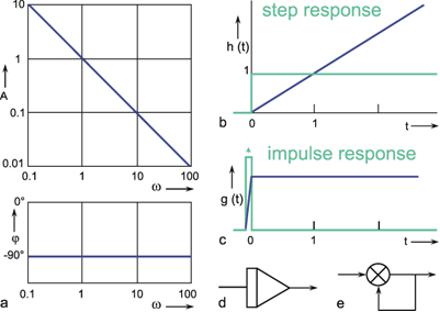
Fig. 4.13 Integrator. (a) Bode plot, A amplitude, ϕ phase, ω angular frequency. (b) step response. (c) Impulse response. In (b) and (c) the input functions are shown by green lines. (d) symbolic representation of an integrator. (e) An integrator can also be realized by a recurrent summation
A mathematically exact integrator can be interpreted as a limiting case of a low-pass filter with an infinitely small corner frequency and an infinitely high amplification. A real integrator could thus be approximated by a low-pass filter with large time constant and large amplification.
In Chapter 4.6 we considered the parallel connection of a low-pass filter and a high-pass filter. Occasionally, in biology we find systems having a step response which seems to consist of two (or more) superimposed exponential functions, i. e., it can be described by a parallel connection of two high-pass filters with different time constants. In a semi-logarithmic plot, this step response can be approximated by two lines with different slopes, corresponding to the two time constants. If the superimposition of more than two exponential functions is necessary for the approximation of the step response, a better interpretation might be obtained by using a power function y = const. t-n. The power function is characterized by the fact that, plotted on a double logarithmic scale, it will show as a line with the slope -n. Mathematically, at the beginning of the step, for t0 = 0 the power function takes an infinite amplitude which, of course, does not apply to realistic systems. If we use the maximum amplitude of the step response A1 at time t1 the power function can be written as y(t) = A1 (t/t1)-n. The amplitude frequency plot of such a system is given by A(ω) = A1Γ(1 - n) (t1 ω)n, whereby Γ stands for the so-called Gamma function (see e. g., Abramowitz and Stegun 1965 ). Thus, the amplitude frequency plot is given by a line with slope n. The phase frequency plot is given by ϕ(ω) = n 90°, i. e., is constant for all frequencies; this holds for 0 < n < 1. For the limiting case n = 1, this system could be interpreted as an ideal differentiator, i. e., as a system which forms the 1st derivative of the input function. The response to a ramp input (x(t) = k t) is given by y(t) = A1 k n/[t1 -n Γ(2 - n)] t1-n.
Figure 4.14 shows the step response of such an "approximate differentiator", namely the mechanoreceptive spine of a cockroach, in a plot with linear coordinates (Fig. 4.14a), and in a double logarithmic plot (Fig. 4.14b). In this case, A1 and t1 correspond to about 450 Hz and 0.02 s, respectively.
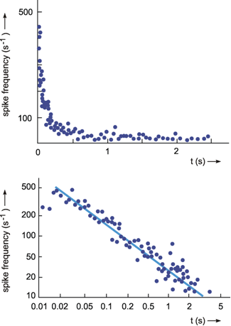
Fig. 4.14 The step response of a cockroach mechanoreceptor, a sensory spine. This response (a), can be approximated by a power function, y(t) = A1 (t/t1)-n, which shows a straight line in a double logarithmic plot (b) (after Chapman and Smith 1963 )
An integrator corresponds qualitatively to a low-pass filter with very low corner frequency and very high gain. A system showing a step response in a form of a power function can be interpreted as an approximate differentiator.
Systems of the 1st order are characterized by the fact that they are endowed with only one energy store (capacitor, spring etc.). If a system has several different energy storage units (e. g., spring and inert mass, see Figure 1.2, or capacitor and inductor in an electrical system), the energy could, under some conditions, be transferred rhythmically from one store to another within the system. This makes the system oscillate. Imagine, for example, giving a short kick to the handle of the mechanical system shown in Figure 1.2. The number of the order of the system corresponds to its number of storage units. (This is also the case for the examples in Chapter 4.3 and 4.4 .)
We will now consider an oscillating system of the 2nd order endowed with low-pass properties (Fig. 4.15). The transfer properties of this system are best described by the step response (Fig. 4.15b). Since the system's amplitude and the duration of oscillations are dependent on an additional parameter, the damping of the system, the step responses are given for different damping values ζ. (For how to determine ζ, see below). In the theoretical case of ζ = 0 (i. e., if the system has no damping) an unlimited continuous oscillation is noted in the frequency ωs = ω0 with a mean amplitude value of 1. ω0 is known as the eigenfrequency or resonance frequency.
If 0 < ζ < 1, a "underdamped" oscillation of the frequency
 is obtained, which decreases to the final amplitude value 1.This would usually be expected to occur in the mechanical system of Figure 1.2.
The envelope of this damped oscillation is an exponential function with the time constant 1/(ζ ω0). Thus, the smaller the damping, the longer will be the transient. For ζ = 1 (the so-called critical damping), the step response approximates the final value 1 without overshoot. For higher damping values (ζ > 1, the "overdamped" case) the curve is even more flattened (i. e., the final value is also obtained without overshoot) but this takes longer than in the case of ζ = 1.This might, for example, happen when the pendulum of the mechanical system of Figure 1.2 is submerged in an oil tank. The exact formulas for these step responses and the corresponding weighting functions are given in the table in Appendix I .
Although for this 2nd order filter, too, a time constant can be given, it cannot be read as easily as that of the step response of a 1st order filter. A practical measure used for the form of the increase of the step response is half-life (HL). This is the time needed by a response to increase to half of its final static value. For a 1st order filter, half-life can be computed simply from the time constant:
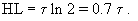
For the 2nd order oscillatory system discussed here, the approximation formula is:
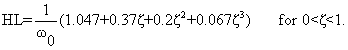
A further useful approximation formula describes the strength of overshoot of the step response. If p denotes the difference between the amplitude value of the first maximum and the static final value,

Figure 4.15 a shows the course of the Bode plot for different damping values ζ. Apart from the formation of a maximum at the frequency ωs, the amplitude frequency plot can be described, as in the case of the non-oscillating 2nd order low-pass filter (Fig. 4.5), by two asymptotes, one being horizontal and a second one exhibiting a slope of -2 on a logarithmic scale. Both asymptotes intersect each other at the eigenfrequency ω0. For ζ = 1, both systems become identical.
The occurrence of a maximum means that the frequencies near ωs are particularly amplified by this system. The over-proportional amplification of this frequency also determines the form of the step response. If damping ζ = 0, the infinitely high maximum occurs at frequency ωs = ω0. With increased damping, the amplitude of the maximum decreases, and its location shifts to lower frequencies (ωs < ω0). If the ζ ≥ 1, a maximum no longer exists. The amplification factor at the eigenfrequency becomes increasingly smaller, while the location of the two asymptotes remains unchanged. The general formula of the amplitude frequency plot is as follows:
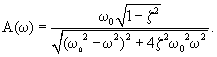
The phase frequency plot is also related to that of a nonoscillating 2nd order low-pass filter (see Fig. 4.5). The maximal phase shift amounts to -180°; at the eigenfrequency, ω0, it takes the value -90°. The greater the damping, the smaller becomes the absolute value of the slope of the phase frequency plot.
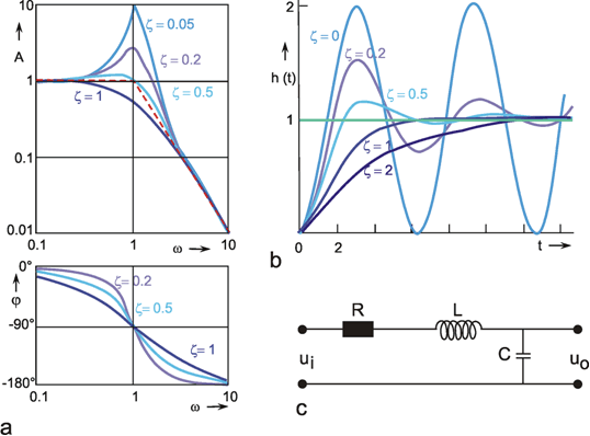
Fig. 4.15 A 2nd order oscillatory low-pass filter. (a) Bode plot, A amplitude, ϕ phase, ω = 2πν angular frequency, ζ, describes the damping factor, where ζ = 0 corresponds to no damping. (b) step response, the input function is shown by green lines.(c) Electrical circuit, R resistor, C capacitor, L inductor, ui input voltage, uo output voltage
Figure 4.15c represents an electronic circuit with the same properties as this system using an ohmic resistor R, an inductor L, and a capacitor C. L and C represent the two energy storages. For this system the following formulas hold:
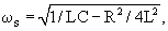
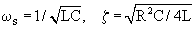 .
.
A mechanical example of an oscillating system of the 2nd order is shown in Figure 1.2. If the parameters of a given 2nd order system are to be obtained quantitatively, the best way is to start by taking the eigenfrequency ω0 from the Bode plot. Value ζ can be obtained by constructing an electronic system of eigenfrequency ω0 and then changing the ohmic resistor until the step response or the Bode plot of the electronic system agree with that of the system under examination. ζ can then be computed from the values of R, C, and L. The simulation of such a filter is explained in Appendix II .
If, in the circuit diagram of Figure 4.15c, the ohmic resistor R and the capacitor C are interchanged, an oscillatory 2nd order system endowed with high-pass properties is obtained. This system will not be discussed further, however.
A system with two different energy storages may oscillate. In terms of low-pass filter properties this corresponds to that of a 2nd order low-pass filter that can show an output function with superimposed oscillation depending on a damping factor.
In the previous sections, a series of different simple systems was addressed from which arbitrarily complex systems could be constructed by combination. In the study of biological systems, however, the reverse problem is normally of interest. Assume that we have obtained the Bode plot of the system under view. The next task would be to describe the measured Bode plot by an appropriate combination of described filters. Once this has been done successfully, the question arises as to the extent to which this model agrees with the biological system in terms of the arrangement of individual elements. That is, to what extent statements can be made about its internal construction in this way.
A general impression of the limitations of this method will be illustrated with the help of very simple examples with known internal structure. Figure 4.16 shows four combinations, each of a high-pass filter and a low-pass filter. Could these four systems be distinguished in terms of their input-output behavior? A comparison of the static part of the step responses of systems c and d shows that in case d static output value will be zero (since the high-pass filter takes the output value zero) while for case c, the output value zero of the high-pass filter is added to the output value of low-pass filter which differs from zero. Both systems can thus be distinguished from each other.
If we look at the static range, it is easy, for this simple case, to predict the step responses for systems a and b. In system a, the high-pass filter produces the static output value zero so that, after some time, the low-pass filter, too, takes the output value zero. In system b, the high-pass filter likewise adapts to zero, after the low-pass filter has reached a static output value (generally different to zero). Systems a, b, and d thus take value zero in the static part of the step response. In this way they can be distinguished from system c, but not from each other.
Systems a and b are linear, whereas system d is endowed with nonlinear properties due to built-in multiplication. If, for this reason, we use step functions of varying amplitudes, the step responses of systems a and b can be calculated by simple multiplication with an appropriate factor that corresponds to the ratio of the related input amplitudes. The responses of system d do not reflect this proportionality (Fig. 4.16e). Thus, while system d exhibits special properties, systems a and b, forming a band-pass filter, cannot be distinguished on the basis of their input-output behavior. Principally, this is not possible for linear systems as the sequence of series connection is irrelevant.
These examples show that, in the study of an unknown system, it is possible to rule out certain combinations (that is, certain hypotheses about the internal structure of a system), but that, on the other hand, a number of different combinations may exist, endowed with the same input-output behavior, which can not, therefore, be distinguished along these lines. A further example of a differently constructed system with the same input-output behavior has already been mentioned (Fig. 4.8).
Especially in the case of linear systems, a decision about the kinds of filters actually involved and about their arrangement can be taken only if a dissection of the total system is possible, and parts of the system can be examined in this way. (On this, see Hassenstein and Reichardt 1953 ). A decision is easier, however, if linear and nonlinear elements occur in a system. This is usually the case in biological systems. For this reason, further examples relating to the analysis of a system will only be dealt with after the discussion of nonlinear elements. Linear systems theory is not superfluous, thought as might be concluded from the foregoing remarks. Rather, it is the prerequisite for understanding nonlinear systems.
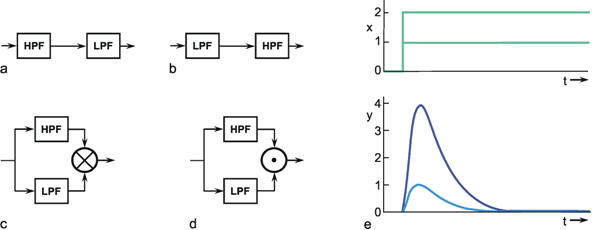
Fig. 4.16 Four combinations of connecting a low-pass filter and a high-pass filter. (a, b) Serial connection, (c, d) parallel connection with summation (c) and multiplication (d). The step responses of (a) and (b) are given in Fig. 4.7, that of system (c), for the case τLPF = τHPF and different gain factors for the high-pass branch in Figs. 4.9b and 4.10b. (e) Two responses to steps of two different amplitudes (green lines) of the system shown in (d) illustrating the nonlinear property of this system (doubling the input amplitude does not lead to twice the output amplitude)
The input-output behavior of a system does not, in many cases, permit a unique conclusion with respect to the internal structure. This is particularly so for linear systems.
This chapter will address the essential properties of nonlinear systems. This requires the introduction of the term characteristic. The characteristic of a system is obtained by measuring the output values y belonging to the corresponding input values x, and then describing the relations between x and y in graphical form. The characteristic is not, therefore, a time function. As an example, the characteristic of a stretch receptor in the abdomen of the crayfish is shown in Figure 5.1. The input value is given by the expansion of the stretch receptor, which is measured in mm. The receptor potential, which is measured in mV, is used as output value.
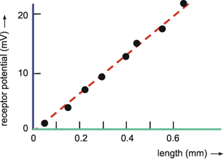
Fig. 5.1 The characteristic describing the dependency of the receptor potential of the crayfish stretch receptor (ordinate: output) on the length of this sense organ (abscissa: input) (after Schmidt 1972 )
The static characteristic constitutes the simplest case. A static characteristic can be used as a good representation of the properties of a system in those cases in which the output succeeds the input without measurable time delay (i. e., in which, for example, no measurable transients occur in the step response. Frequently, however, the output function requires a certain time until it has caught up with the input value. This applies to all systems that are endowed with an energy store (e. g., spring, inert mass, capacitor); that is, to all systems of the 1st and higher orders. (Systems without energy storage are therefore also known as systems of the zeroth order). In such cases dynamic characteristics may be obtained; they are discussed in Chapter 5.3 .
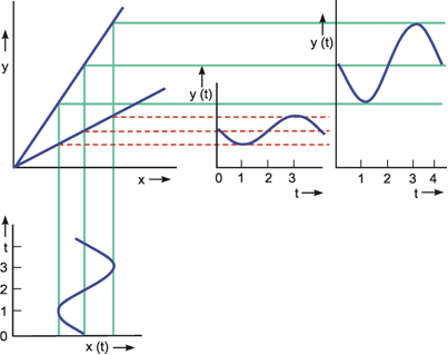
Fig. 5.2 The construction of the output function y(t) for a given input function x(t), shown for two different linear characteristics
If the static characteristic of a system of the zeroth order is known, the response of this system to an arbitrary input function can be obtained graphically by a "reflection along the characteristics." This is shown in Figure 5.2 for two linear characteristics with different slopes. The input function x(t) is plotted relative to the characteristic such that the ordinate x(t) of the input function lies parallel to the abscissa x of the characteristic. The coordinate system for the output function y(t) is arranged such that its ordinate y(t) lies parallel to the ordinate y of the characteristic. The amplitude value of the output function can then be obtained for every moment of time by reflection of the amplitude value of the input function along the characteristic. The corresponding abscissa value t of the input function is again marked off the abscissa of the output function. (For the case of a curved, i. e., nonlinear, characteristic, this is shown for three selected points in Figure 5.3). For systems for the 1st and higher orders, this construction is possible only if transients are of such short duration that they are negligible in terms of the desired precision, or if only the static behavior of the system is of interest.
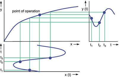
Fig. 5.3 The construction of the output function y(t) for a given input function x(t), shown for a nonlinear (in this case logarithmic) characteristic. As example, three time values t1, t2, and t3 are marked. The point of operation is defined as the mean of the input function (after Varju 1977 )
The comparison of the two characteristics presented in Figure 5.2 shows that the steeper the slope of the characteristic, the greater is the amplification of the system. The slope of the characteristic thus reflects the amplification factor of the system. If the line does not cross the origin, or if the characteristic is nonlinear, the amplification A = y/x is not identical with the slope of the characteristic.
Rather, the relation of input and output amplitude (i. e., the amplification factor of the system) changes with the size of the input value. For the characteristic shown in Figure 5.3, for example, the amplification for small input amplitudes is large, whereas it continues to decrease with increasing input amplitudes. To enable us to describe the range of the characteristic in which the values of the input function are located ("range of operation"), the point of operation is defined as that point of the characteristic which corresponds to the mean of the input function (Fig. 5.3). In addition, the term modulation is used here to characterize the transfer properties of a system. The modulation of a function means the ratio between amplitude and mean value of the function.
The great majority of characteristics occurring in biology are nonlinear; that is, they cannot be described by simple proportionality. In sensory physiology, for example, only a few receptors are known which are linear within a large range. One such case is shown in Figure 5.1. Many nonlinear characteristics can be approximated by a logarithmic or an exponential characteristic, at least within a given range.
The logarithmic characteristic y = const ln (x/x0) constitutes the mathematical form of the so-called Weber-Fechner Law. This states that in a number of sense organs the response y is proportional to the logarithm of the stimulus intensity x. If x ≤ x0, the response takes value zero. X0 is therefore known as threshold intensity. The simplest way to check whether a characteristic actually takes a logarithmic form, is to transfer it to a semilogarithmic scale, which should produce a straight line. This is shown in Figure 5.4 by using as an example a sensory cell of a turtle's eye. A logarithmic relation between light intensity I and receptor potential A can only be found for a limited range of about two orders of magnitude. Above and below this range, there are deviations from the logarithmic course (i. e., in this representation, from the line).
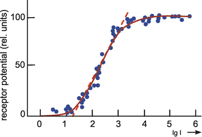
Fig. 5.4 The dependency of the receptor potential of a retinal sensory cell of a turtle (ordinate) on the intensity of the light stimulus (abscissa, logarithmic scale). The central part can be approximated by a straight line (dashed), indicating the logarithmic part of the characteristic (after Schmidt 1973 )
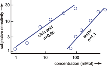
Fig. 5.5 The subjective sensitivity of tasting the concentration of citric acid and sugar of human subjects (double logarithmic scales). n gives the slopes of the lines which correspond to the exponents of the underlying power functions (after Schmidt 1973 )
The power characteristic y = const (x - x0)n is the mathematical form of the Power Law or Stevens' Law. x0, in turn, denotes the threshold value, i. e., the value that has to be exceeded at the input in order to get a measurable response at the output. For the power characteristics measured in biology, the exponents occur between 0.3 < n < 3.5. A power characteristic is present if this characteristic results in a line after double - logarithmic plotting. The slope of this line takes the value n. Two examples are shown in Figure 5.5. These describe the intensity of subjective sensations of taste in sampling various concentrations of citric acid and sugar solutions. Figure 5.6 is a schematic illustration of the course of the power function on a linear scale with three different exponents. A linear characteristic is obtained if n = 1.
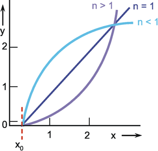
Fig. 5.6 Three power functions plotted on linear scales. x0 describes a threshold value, n is the exponent of the power function. x input, y output
The example of the logarithmic characteristic, as shown in Figure 5.7, illustrates the most important transfer properties of nonlinear static characteristics. Figure 5.7a shows the sine responses obtained by "reflection" at the characteristic as already shown in Figure 5.3, but now with four different input amplitudes, and a fixed point of operation. The first property we notice is that the sine function is highly distorted. This shows that the output function is endowed with a number of harmonics in the sense of Fourier analysis, which do not occur in the input function, the latter being a pure sine function. This is also known as a change of the degree of harmonic distortion. This distortion is accompanied by a shift in the mean. Since the proportion of the area below the line, which runs at the level of the point of operation, becomes larger with increasing amplitudes, the mean of the output function decreases. Thus, as a function of the size of input amplitude, a shift in the mean ("dc-shift") is observed. On account of this dc-shift and the distortion of the amplitude, the degree of modulation also changes as a result of the transfer by nonlinear characteristics.
As shown in Figure 5.7b, these quantities change even if the amplitude of the input function, though not the point of operation, is kept constant. With respect to systems to be discussed later, it should be noted that with these nonlinear static characteristics, the response to a symmetrical input function (symmetrical in terms of a vertical axis through a minimum or maximum) is again symmetrical. This is not true for certain combinations of other systems, for example nonlinear static characteristics and linear filters addressed below.
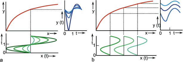
Fig. 5.7 The effects of a nonlinear transformation. (a) Effects of changing the input amplitude. (b) Effects of changing the point of operation. x(t) input function, y(t) output function (after Varju 1977 )
If the form of a nonlinear characteristic shows no discontinuity in the slope, but only a smoothly changing slope, this may be called soft nonlinearity. This applies to the logarithmic and the exponential characteristic as long as the course of the input function stays above the threshold value. By contrast, those characteristics that show a discontinuous slope may be called hard nonlinearities. A hard characteristic in the strict sense does not occur in biology since the edge will, in reality, always tend to be more or less rounded down. The difference between a hard and soft characteristic is thus gradual. In the field of technology, such hard characteristics are more marked. Below, some of these hard characteristics will be described to the extent they are endowed with properties which may also play a role in biological systems. The typical effect of each characteristic will be illustrated in the way that the various response are drawn using an appropriately chosen sine function as input function.
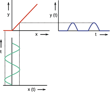
Fig. 5.8 The characteristic of a rectifier. Negative input values are made to zero. x(t) input function, y(t) output function
Figure 5.8 shows the diode or rectifier characteristic. This has the effect that all negative input values take zero at the output. For a sine function with the mean value zero, all negative half-waves are thus cut off. The positive halfwaves are transmitted without any disturbance. Therefore it is also called the half-wave rectifier. If a range of operation is used that comprises only positive input values, the nonlinear property of this characteristic cannot be identified.
For a characteristic with saturation (Fig. 5.9), the output values remain constant, once the absolute value of the input has exceeded a certain value, the "saturation value" xs. If the amplitude of a sine function at the input oscillation is thus sufficiently large, the extreme values of the sine curve are flattened due to this nonlinearity.
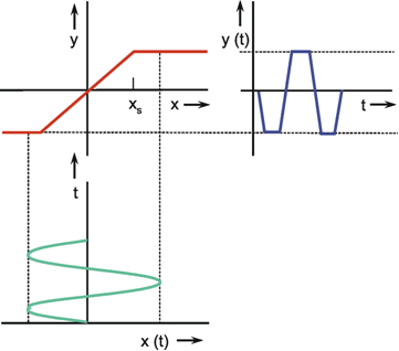
Fig. 5.9 A characteristic with saturation. When the input exceeds a given value xs the output does not increase further. x(t) input function, y(t) output function.
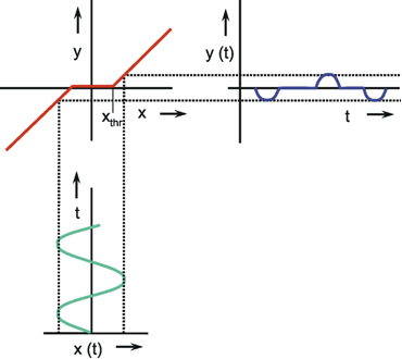
Fig. 5.10 Characteristic with threshold. The input value has to exceed a value xthr, before the output value changes. x(t) input function, y(t) output function
If the characteristic is endowed with a threshold, usually known as a dead zone in the technical literature, the input quantity must first exceed a certain threshold value xthr in order to show an output value that is different from zero (Fig. 5.10). In this case, only the values of the input function above the threshold are thus transmitted. As with the rectifier characteristic, those input functions whose values are all above the threshold are transferred without any disturbance.
In biology, a combination is frequently found of the properties of the characteristics shown in Figures 5.8 to 5.10. For example, each sensory cell is endowed with a certain threshold as well as an upper limit. The subsequent synapses have a rectifying effect. The result is a characteristic whose general form can be approximated by three asymptotes, as shown in Figure 5.11. One example of such a characteristic is shown in Figure 5.4, although in this case, the ascending part follows a logarithmic rather than a linear course. It should also be mentioned that this characteristic is described by the function y = A0 I/(IW + I). This function is shown as a solid line in Figure 5.4, with I being plotted logarithmically. A0 denotes the distance between the two horizontal asymptotes. The turning point is at Iw/0.5 A0. The asymptote, shown as a dashed line in Figure 5.4, is described by the formula y = const. log I/Ithr. Here, Ithr, denotes the theoretical threshold value at which this asymptote cuts the zero line. As can be seen in Figure 5.4, the actual threshold value is lower, since this characteristic does not exhibit a discontinuous slope. Characteristics of this form are also known as sigmoid characteristics. Another often used form of a sigmoid characteristic is the "logistic" function y = 1 /(1 + e-ax). The parameter a describes the slope of the function (Fig. 5.11 b). This function uses the range between 0 and 1 on the ordinate. If the same function is spread to the range between -1 and 1, it is given by tanh ax.
The characteristic of a so-called ideal relay (Fig. 5.12) enables only two discrete output values, depending on whether the input value is located above or below a critical value (in this case zero). This characteristic thus describes an all-or-none effect. A function of this form is also called the Heaviside function.
The characteristic of a full-wave rectifier (Fig. 5.13) transmits the absolute value of the input function (i. e., the negative half-waves of the sine function are reflected along the abscissa). If the input function is placed symmetrically in relation to the zero point, the frequency of the fundamental of the output function is doubled by this characteristic, compared to the input function.
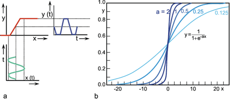
Fig. 5.11 (a) A combination of a rectifier, a threshold, and a saturation, as it is often found in biological systems (see Fig. 5.4). (b) A sigmoid characteristic corresponding to the logistic function, parameter a is a measure for the slope of the function. x(t) input function, y(t) output function
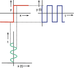
Fig. 5.12 An all-or-none characteristic corresponding to the Heaviside function. x(t) input function, y(t) output function
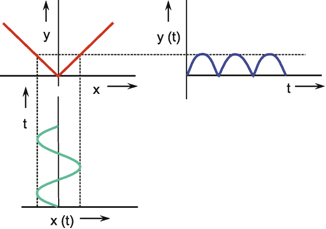
Fig. 5.13 The characteristic of a full-wave rectifier. Negative input values are made positive. x(t) input function, y(t) output function
With the exception of the full-wave rectifier, all the characteristics discussed so far are endowed with a monotonously ascending course; that is, their slope is always greater than, or equal to zero. A further example of a nonmonotonous characteristic is shown in Figure 5.14. As in the case of the two-way rectifier, an appropriate choice of range of operation will enable generation of a doubling of the fundamental frequency, or a phase shift of 180°. This occurs when the point of operation is changed from a to c in Figure 5.14. A doubling of frequency may occur when the point of operation lies at about position b. An example of a nonmonotonous characteristic of a biological system is shown in Figure 5.15.
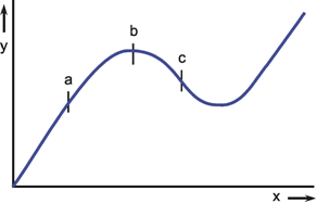
Fig. 5.14 A nonmonotonuous characteristic. a, b, and c mark three points of operation. x input, y output
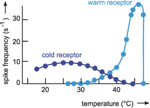
Fig. 5.15 The discharge rate of cold receptors and warm receptors of the cat at different temperatures (tonic part of the responses). In general, a given spike frequency can represent two different temperature values (after Schmidt 1973 )
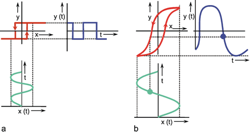
Fig. 5.16 The characteristics of a realistic relay (a) and of a hysteresis (b). In both cases, for a given input value the value of the output depends on the actual history, i. e., of how this input value was approached. This is symbolized by the arrows. x(t) input function, y(t) output function
In addition to exhibiting properties described as soft-hard, monotonous - nonmonotonous, static nonlinear characteristics can also be distinguished as univalued or multivalued. Unlike the univalued characteristics discussed so far, a multivalued characteristic is endowed with more than one output value corresponding to any one particular input value.
In a realistic relay, the value at which the switch is closed with increasing voltage usually differs from the value at which, during the drop in the voltage, the switch is opened again. The result is the multivalued characteristic of a realistic relay (Fig. 5.16a). This characteristic thus consists of two branches. Which of the two happens to apply at the time depends on the actual history; that is, on whether the input values happen to be increasing or decreasing. The temporal course is indicated by arrows. As with an ideal relay, only two discrete values are obtained at the output. Another characteristic of this type is the so-called hysteresis which matches the form of magnetization effects found in physics (Fig. 5.16b).
The transfer properties of a static characteristic can be illustrated by "reflecting" the input function at the characteristic to obtain the output function. Nonlinear characteristics distort the signal by increasing the content of higher harmonics. They can change the mean value (dc shift). Different types of static nonlinear characteristics may be grouped as soft - hard, monotonous - nonmonotonous, and univalued - multivalued.
Systems of the 1st and higher orders (i. e., systems with energy storage units) exhibit a typical transition behavior, for example in the case of the step response, until they reach a final output value. This transition during a constant input value (e. g., after a step or an impulse) is known as the dynamic part of the response or the transient. After the dynamic part fades, the stationary part of the response is obtained. This stationary part can be represented by a constant output value, as in the simple case of a first order filter. It is then also known as the static part. In undamped oscillatory systems of higher order (Fig. 4.15b) or in particular feedback systems (see Chapter 8.6 ), the stationary part may also be nonstatic. In these examples the stationary part of the response can be represented by infinitely continuing oscillations of a constant amplitude, i. e., it is periodic.
When applied to examples of tonic and phasic sensory cells, the dynamic part of the response of the phasic sensory cell to an ascending step thus exhibits a rapidly ascending increase initially, and then descends more slowly. In the case of a tonic sensory cell it consists of an ascending course. For the tonic sensory cell, the stationary part (in this case the static one, too) takes a higher value than the initial one, whereas for the phasic sensory cell, it remains at the level of the initial value.
Determination of the characteristic of a system endowed with dynamic properties poses a number of problems. This is demonstrated by the step response of a 1st order low-pass filter (solid lines) shown in Figure 5.17a together with the input step (dashed line). If one wants to read the output value corresponding to a particular input value x, a different value is obtained for each of the four selected time values t1 to t4. If the experiment is repeated with further step functions of varying amplitudes, a linear characteristic is obtained for each selected time ti, but these characteristics differ from another (Fig. 5.17b). Only after the dynamic part is finished (t
 ) is a fixed characteristic obtained whose slope indicates the static amplification factor. During the dynamic part, the amplification factor changes continuously.
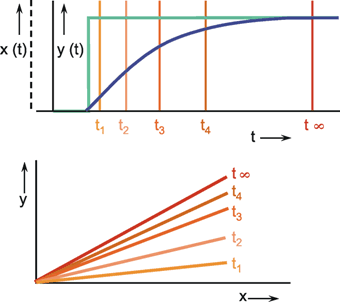
Fig. 5.17 Example for a linear dynamic characteristic. (a) Step input (green line) and step response (blue line) of a 1st order low-pass filter. Relating input and output of this filter yields different characteristics for each moment of time. These characteristics are shown for four selected time values t1 – t4, and for t
 in (b). x(t) input function, y(t) output function (after
Varju 1977
)
in (b). x(t) input function, y(t) output function (after
Varju 1977
)
The dynamic characteristic of a system endowed with an energy store is thus not represented by a single curve, but rather a set with t as a parameter. Although the characteristic obtained for t
 is also known as the static characteristic of the dynamic system, construction of the output function by reflection at the characteristic is not possible in this case. The simplest way to obtain the response of a system endowed with a known dynamic characteristic is by simulation using electronic circuits or digital computers.
In Chapter 4 the amplification factors were mostly set at k = 1 for reasons of clarity. Since we have to distinguish between static and dynamic amplification factors, which was not explained in detail earlier, this can now be summarized as follows: the step response of the 1st order low-pass filter is h(t) = k (1 - e-t/τ). Here, k corresponds to the static amplification factor described above. It agrees with the ordinate value of the horizontal asymptote of the amplitude frequency plot. The step response of the 1st order high-pass filter is h(t) = kd e-t/τ. The static amplification factor of a high-pass filter is always zero. kd is the maximum dynamic amplification factor. It indicates the maximum amplitude of the step response, provided this is not influenced by low-pass properties of the system. kd, too, agrees with the ordinate value of the horizontal asymptote of the amplitude frequency plot.
For a dynamic system, there is not just one characteristic but a set of characteristics, one for each time value. In nonlinear cases, the easiest way to illustrate the transfer properties of such a dynamic characteristic is to use a simulation.
So far only the properties of some nonlinear characteristics have been discussed. Since combinations of static nonlinear characteristics and linear filters are relatively easy to understand, some of them will be addressed below.
In a serial connection of a linear filter and a nonlinear system, the form of the output function depends essentially on the sequence of the two elements. For this reason, Chapter 6.1 will examine the sequence, linear element - nonlinear element, and Chapter 6.2 the converse sequence, nonlinear element - linear element.
To begin with, we will look at a system consisting of a low-pass filter and a nonlinear static characteristic connected in series, as shown schematically in Figure 6.1. Sine functions of low frequency at the input (x) of the low-pass filter result in high amplitudes at its output (z) and thus, at the same time, at the input of the nonlinear element. The higher the amplitude, the greater is the distortion by the nonlinear characteristic. This changes the mean of the output function and the amount of higher harmonics. High frequency sine functions at the input (x), result in low amplitudes at (z). Accordingly, the nonlinearity produces only slight distortions and slight shifts in the mean at (y).
In all cases, however, the sine responses constitute functions that are symmetrical in relation to a vertical axis through an extreme point of the function. If, accordingly, a high-pass filter is combined with a nonlinear element, the transfer properties of the total system are produced in an analogous way.
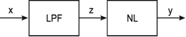
Fig. 6.1 Serial connection of a linear filter (e. g., a low-pass filter) and a nonlinear characteristic
If the linear filter is serially connected to the nonlinear one in the reverse order, different properties will result, since the harmonics, first produced by the nonlinear element, will undergo a variety of phase shifts, depending on a frequency of the subsequent linear filter. As a consequence, the output function can become asymmetrical in relation to a vertical axis through an extreme point. Figure 6.2 and 6.3 show the sine responses of such systems for different forms of characteristics and different nonlinear filters. In addition to the input function x(t) and the output function y(t), the output function of the nonlinear characteristic z(t) is also shown.
It should be mentioned, however, that one may not necessarily infer a series connection of a nonlinear characteristic and a linear filter from such an asymmetrical response to a sine function. Dynamic characteristics and multivalued nonlinear static characteristics can also produce such asymmetrical sine responses. (See the example shown in Figure 8.16). Those interested in a more detailed discussion of these systems are referred to the literature (e. g., Varju 1977 ).
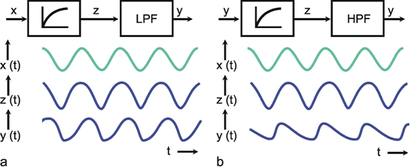
Fig. 6.2 Serial connection of a nonlinear characteristic and a linear low-pass filter (a) or a high-pass filter (b). The nonlinear characteristic is described by a function z = √ x, x(t) input function, y(t) output function. z(t) describes the output of the first system
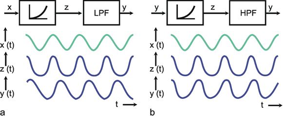
Fig. 6.3 Serial connection of a nonlinear characteristic and a linear filter as in Fig. 6.2, but with a nonlinear characteristic following the function z = x2. x(t) input function, y(t) output function. z(t) describes the output of the first system
A further example of the series connection of linear filters and nonlinearities is provided by a system that occurs quite frequently in biology. Some sensory cells, for example, respond only to an ascending, but not descending, stimulus. This means that the system responds only if the first derivative of the input function is positive. This system is called an "unidirectional sensitivity unit." Such a system is practical only if an adaptive system (that is, a high-pass filter) is serially connected to this unit. Otherwise, the output value, when responding to an alternately ascending and descending input function, would quickly approach an upper limit since only the ascending parts of the function exhibit a response.
Such a system may be present, for example, if a transfer of information is effected by the release of a chemical substance (synaptic transmitters, hormones). As the input value increases, there is a growing concentration of this chemical substance; but with a decreasing input value, the concentration of the substance does not decrease accordingly, but may be reduced quite slowly (e. g., by diffusion or by a catabolic mechanism, producing an exponential decay). This corresponds to a serial connection of a unidirectional sensitivity element and a high-pass filter. This has become known as a "unidirectional rate sensitivity (URS)" (see Clynes 1968 ).
Figure 6.4 shows the response of this system to a triangular function. Due to the positive slope, the ascending part of the triangular function is transmitted unchanged by the unidirectional sensitivity element. At the output, the following high-pass filter thus shows a typical ramp response (Fig. 4.3). For this reason, an exponential function is obtained which, if the ramp lasts long enough, ascends with the time constant τ of the high-pass filter to a plateau whose height is proportional to τ and the slope of the triangular function (ramp response, Fig. 4.3d). During the descent of the triangular function, a constant value is produced at the output of the unidirectional sensitivity element. Together with the time constant τ, the output value of the high-pass filter thus descends again to zero. If one shortens the ramp duration with the amplitude remaining unchanged, however, there is no longer sufficient time to attain the new plateau after ascending, or the zero line after descending. After a certain transient period, the ascending and descending parts are again antisymmetrical relative to each other. The mean of the output function shifts, however, as a function of the frequency (dc shift), as shown in Figure 6.4. This shows another qualitative property of a serial connection of a nonlinear element followed by a linear element. It is possible that there is a dc shift of the output signal, the size of which depends on the frequency of the input signal.
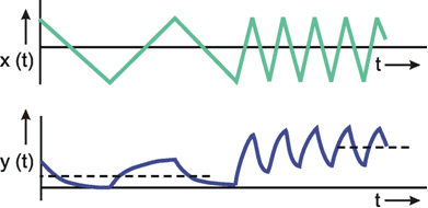
Fig. 6.4 Ramp responses of an unidirectional rate sensitivity system. This system responds only to those parts of the input function which have a positive slope. The subsequent high-pass filter determines the form of the response (ramp response, Fig. 4.3). When the frequency of the fundamental wave of the input function increases, the mean value of the output function (thin dashed lines) increases, too (after Milsum 1966 )
When a system contains serially connected linear and nonlinear elements, then, depending on the order of the sequence, qualitative differences can be found with respect to its transfer properties. When the static nonlinear element is followed by a linear element, symmetrical input functions (e. g., sine functions) can be transformed to asymmetric forms; or, depending on the frequency of the input function, a dc shift of the output function could occur. This is not possible where the elements are in reverse order.
There are no general rules for study of nonlinear systems, since there is, as yet, no unified theory of nonlinear systems. Below, we will therefore describe several methods for the study of nonlinear systems, which should be considered no more than a collection of approaches.
First, it is important to check whether the system to be studied is linear or not. The simplest test is to examine the responses to steps of different amplitudes. Nonlinearity is present if a nonlinear relation between input and output is observed. However, the opposite is no proof of linearity of a system, though, as can be seen by examining the system shown in Figure 6.4. A better, though more difficult, test consists of studying the responses to sine functions of different frequencies and amplitudes. If the corresponding response functions turn out again to be sine waves in each case, the system is linear.
Once it is established that the system examined is of a nonlinear nature, one could try to simplify the problem by searching for a linear approximation to the system. If it is endowed with a nonlinear characteristic, one could try to undertake a "linearization" of the system by using only small input amplitudes, if possible. As Figure 5.7 shows, an approximation to the linear case can always be obtained with soft characteristics. By changing the position of the point of operation, a nonlinearity can be divided into several small linear segments. As an example, Figure 7.1 shows the result of an investigation of a position reflex. (A detailed description of this system is given in Chapter 8.4 .) Whereas the response to the input function of a large amplitude differs clearly from the form of a sine function, the response to a small amplitude function is very similar to a sine function. When the system that is being studied is linear at least for selected ranges, a "linearization" can often be realized by first examining only the linear range.
In case of hard nonlinearities, a linearization can be obtained in a simple way only if an appropriate choice can be made regarding the point of operation. For example, the nonlinearity of the system shown in Figure 6.4 cannot be linearized for sine function at the input. By contrast, a linearization for a step function at the input is possible, as this function contains no descending parts. (For other possibilities of linearization of such nonlinearities see Spekreijse and Ousting 1970 ).
If the system is endowed with a distinct dynamic characteristic, it is useful, first, to study the static behavior of the system (see Chapter 5.3 ). Once the static properties are known, the subsequent study of the dynamic properties will be less complex.
As we have seen in the previous sections, many nonlinear systems provide an asymmetrically distorted sine response. The Bode plot of such a system would be difficult to measure because the phase frequency plot cannot be determined exactly since a phase angle is defined only between two functions of the same type, e. g., two sine functions. If a reduction in amplitude does not produce a sufficient linearization (i. e., a sine function at the output) one option would be to study just the fundamental wave of the output function (see Chapter 3 ) and then to construct the Bode plot for this. Some mathematical operations are required, though, to determine the fundamental wave of the output function.
As mentioned earlier, for linear systems various input functions provide the same information about the system. Since this does not apply to nonlinear systems, it is possible that, with each of these input functions, different information will be obtained.
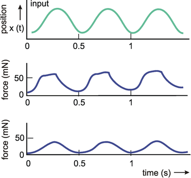
Fig. 7.1 "Linearization" by means of small input amplitudes. The example shows the investigation of a position reflex (see also Fig. 8.6). The upper trace shows the input function (position). The two lower traces show responses (force) for sine wave inputs of different amplitude, namely 0.3 mm, above, and 0.08 mm, below. The response resembles a sine function much better in the second case compared to the first.
As the example in Chapter 6.3 has already shown, it is quite conceivable that a specific property of the system can only be identified when using one particular input function, but not with another. For this reason, it is necessary in studying nonlinear systems that the responses to as many different input functions as possible should be considered. In order to characterize the system as completely as possible, the amplitude (in particular) in addition to the type of input function, should be varied within the widest possible range.
An input function that is sometimes used in the study of nonlinear systems, and which has not been mentioned so far, is the double impulse (i. e., two successive impulses with a short interval between). In a linear system the responses to the two parts of the function would add up linearly. From the type of additivity found in a nonlinear system, it is also possible to draw conclusions about the underlying elements. Analogously, the double step - two successive step functions - can be used. For a more detailed study of this method, the reader is referred to the literature ( Varju 1977 ).
The more complicated, and thus harder to comprehend, the systems under view tend to be, the more it is necessary to accompany experimental investigation by a simulation of the system. This is especially true for the study of dynamic nonlinear characteristics. First, on the basis of initial experimental findings, a hypothesis is made about the structure of the system. This hypothetical system is then simulated by way of electronic circuits or digital computer programs. The hypothesis is tested, and modified if necessary, by comparing the responses of the real and the simulated systems. This procedure is repeated until the behavior of the model agrees with that of the biological system in terms of the desired degree of accuracy. Simulation is not an end in itself; rather, in its course, a number of insights, relevant to the further study of the system will result.
Experience has shown that, in attempts to formulate a merely qualitative hypothesis of a system's construction on the basis of its initial study, such a qualitative interpretation may easily contain unnoticed errors, e.g., by overlooking some inconsistencies. This is especially true if nonlinear properties are present, since their influences on the behavior of the total system are often hard to assess. By making a quantitative hypothesis, needed for the design of a simulation model, such errors are far more likely to be recognized. When realizing the simulation, at the least, one is obliged to formulate an elaborately developed hypothesis, which can then also be tested, quantitatively.
If agreement is found between model and system, it is relatively easy (on the basis of the known model, and by a systematic selection of new input functions) to discover new experiments suited to testing the hypothesis even more thoroughly, and thus making it more reliable. On the other hand, if inconsistencies between the real system and the model are found, which is usually the case it is now possible, since the discrepancies can be clearly defined, to modify the hypothesis, and thus the model, to ensure an improved description of the system. If, in the course of this procedure, two alternative hypotheses emerge, both of which agree with the results obtained so far, input functions can be selected, on the basis of the models, that will help to distinguish between the two hypotheses. In any case, the simulation is thus a heuristically valuable tool in the study of a real system.
Once a simulation has been achieved with the desired degree of accuracy, the model will provide a concise description both of the different experimental data and of the real system. Moreover, the model will come in useful when the response of the system is sought to input functions that have not previously been examined in detail, and whose investigation within the framework of the real system would be too complicated. The unknown response to the system can be obtained quickly and easily by using the model. One example of this is the study of processes covering an extremely long time period. Their simulation can be conducted more speedily.
If the simulation has been concluded successfully in the sense that the responses to a large number of greatly varied input functions can be simulated by means of a unified model, it may ultimately be assumed that the essential properties of the real system have been most probably identified and described.
There is no systematic procedure for investigating nonlinear systems. Rather, a number of rules have to be considered. Simulation is an important tool which can provide a concise description of the system and, more importantly can help to design new experiments.
An Example: The Optomotor Response
A classic example of a nonlinear system is the optomotor response investigated by Hassenstein, Reichardt, and colleagues ( Hassenstein 1958a , b , 1959 , 1966 ; Hassenstein and Reichardt 1956 ; Reichardt 1957 , 1973 ). If a visually oriented animal is placed in the center of an optically structured cylinder, which, for example, contains vertical stripes, and this cylinder is rotated around its vertical axis, the animal tries to move its eyes with the moving environment. This can result in nystagmus-like eye movements (e. g., in humans) or in movements of the head or of the whole body (as in insects, for instance). The biological sense of this optomotor response is assumed to be an attempt keep the sensory environment constant.
In most experiments, the animal is held in a fixed position, and its turning tendency is measured in different ways, for example by recording the forces by which the animal tries to turn. When both eyes, or at least a large part of one eye, are regarded as one input channel, and the turning tendency is measured as output, the whole system can be considered as a band-pass filter (see Box 1 ).
The eyes of insects, however, consists of a large number of small units, the ommatidia. It is possible to stimulate neighboring ommatidia with independent step functions by changing the light intensities projected onto separate ommatidia. Using this technique, it was shown that, in order to detect the movement of the visual pattern, stimulation of two neighboring ommatidia of an eye is sufficient. Thus, for a more detailed analysis, a system can be considered that has two inputs (two ommatidia called O1 and O2) and one output channel (the turning tendency TT, Figure B2.1). For this system, where the first intensively studied object was the beetle Chlorophanus, the following results could be obtained.
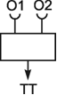
Fig. B 2.1 The elementary movement detector. Two ommatidia, O1 and O2, form the input; the turning tendency TT represents the output of the system
The two ommatidia were stimulated by optical step functions, i. e., by a stepwise increase or decrease in the light intensity. It could be shown that the absolute value of the light intensity of the step functions was not relevant over a wide range; only the size of the intensity change influenced the turning behavior of the animals. This indicates that only a high-pass filtered version of the input function is processed. This is shown by the two high-pass filters in Figure B2.3.
When two neighboring ommatidia O1 and O2 are stimulated with consecutive positive steps, i. e., by increasing the light intensity at O1 and, after a delay, at O2, a reaction following the apparent movement (O1 → O2) was observed. The same reaction was obtained when these ommatidia were stimulated by consecutive negative steps, i. e., with decreasing light intensity. This is shown in the Table B2.2 where this movement direction is shown as positive. When, however, the first ommatidium received a positive step and, consecutively, the second ommatidium a negative step, the animal tried to move in the opposite direction. This means that the direction of the apparent movement was reversed (O2 → O1), which is shown by negative signs in Table B2.2. The same result was obtained when the first step was negative and the second positive. These results are summarized in Table B2.2. The comparison of the signs indicates that some kind of multiplication takes place between the two input channels (Fig. B2.3).

Fig. B 2.2 The table shows the behavior of the system in qualitative terms. The stimulation of the ommatidia is marked by a positive sign, when the light intensity is increased, and by a negative sign, when it is decreased. In all cases, O2 is stimulated after O1. The turning tendency TT is positive when the movement follows the sequence of the stimulus, i. e., from O1 to O2, and negative, when the animal turns in the opposite direction
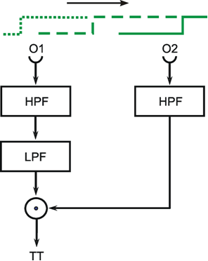
Fig. B 2.3 A simple version of a movement detector which responds to movements from left to right, i. e., from O1 to O2 (see arrow). LPF: low-pass filter, HPF: high-pass filter
However, a direct multiplication of the high-pass filter output signals does not agree with the following results. When the neighboring ommatidia O1 and O2 were stimulated with consecutive positive steps, but the delay between the two steps varied, the intensity of the reaction depended on the duration of the delay, being small for very short delays, strongest for a delay of about 0.25 s, and again decreasing for longer delays, but still detectable for a delay of up to 10 s. This means that the multiplication provides a zero result when the signal in the first input channel occurs at the same time as that of the second input channel. Multiplication provides the highest value when the first signal advances the second by about 0.25 s and the result steadily decreases if the delay increases further. This result is obtained when we assume that the signal from the first ommatidium, O1, having passed the high-pass filter, is transmitted by a low-pass filter. The resulting band-pass response is then multiplied by the signal of the second channel, O2 (Fig. B2.3). This hypothesis was supported by a number of control experiments ( Hassenstein 1966 ). Thus, the elementary movement detector could be shown to consist of two parallel channels containing linear elements, and a nonlinear calculation, namely a multiplication, of the signals of the two channels as shown in Figure B2.3.
It is not shown in Figure B2.3 that the real system, of course, consists of more than two such ommatidia, rather, the output of a large number of such elementary movement detectors is summed to produce the optomotor response. Furthermore, in addition to the movement detector monitoring the movement in the direction from O1 to O2, mirror image detectors monitor the movement in the reverse direction.
The properties of this movement detector could also be interpreted in the following way. Two input functions x1(t) and x2(t) are measured by the two ommatidia O1 and O2, respectively. For a relative movement between the eye and the environment, both ommatidia receive the same input function, except for a time delay Δt which depends on the relative speed. Thus, the input of the second ommatidium x2(t) equals x1(t+Δt). If, for the sake of simplicity, we neglect the transfer properties of the
filters before the multiplication, the output signal corresponds to the product x1(t) x2(t) = x1(t) x1(t + Δt). This signal is not directly fed to the motor output, but is first given to a low-pass filter with a great time constant (not shown in Figure B2.3). As this low-pass filter can be approximated by an integrator ( Chapter 4.8 ), the actual turning tendency might be described by TT = ∫ x1(t) x1(t + Δt) dt. This corresponds to the computation of the correlation between the two input functions. The correlation is higher, the more similar both functions are, which means the smaller Δt is, which, in turn, means the higher the speed of the movement. Thus, the movement detector, by determining the degree of correlation between the two input functions, provides a measure of speed.
There are two ways of assigning a desired value to a variable, such as the position of a leg or the speed of a motor car-to give a biological and a technical example. One way of doing this is by the so-called open loop control. It requires knowledge as to which value of the controlling variable (input value) corresponds to desired value of the controlled variable. For the first example, this would be the connection between the spike frequency of the corresponding motor neurons (input) and the leg position (output), and for the second, technical example, it would be the connection between the position of the throttle and the driving speed. After adjusting the appropriate controlling variable, the correct final value is normally obtained.
If the value of the variable is influenced by some unpredictable disturbance, (e. g., by a force acting of the leg, or, in the case of the moving car, by a speed-reducing head wind) the effect of such a disturbance cannot be compensated for by such an open loop control system. Open loop control, therefore, presumably occurs in cases where no such disturbances are expected. For example the translation of a spike frequency into tension of a muscle, if we disregard effects like fatigue, or, in the case of a sensory cell, the transformation of the stimulus intensity into electrical potentials, thus correspond to an open loop control process.
If disturbances are to expected it is, however, sensible to control the value of the output variable via a closed loop control. This is done by using a feedback system. In this sense, a feedback control system is a system designed to keep a quantity as constant as possible in spite of the external influences (disturbances) that may affect it. It will be explained below how a feedback control system can eliminate, or at least reduce, the effect of such unpredictable disturbances.
In contrast to an open loop system, a closed loop system or feedback system may compensate effects of external disturbances.
Before describing in detail the functioning of a feedback control system, the most important terms required for this will be presented schematically (Fig. 8.1), and using a highly simplified example, namely the pupil feedback system. (A detailed description of this system is found in Milsum (1966) , for morphological and physiological details see Kandel et al. 1991 .) The pupil feedback system controls the amount of light reaching the retina of the eye by reducing the diameter of the pupil, via the iris muscles, as illumination of the retina increases. As illumination decreases, the size of the pupil increases accordingly. The controlled variable, whose value should be kept as constant as possible, despite the effect of external influences (here the illumination of the retina) is called output variable or control variable. This is the output variable of the total "feedback control system".
The value taken by the output variable, the so-called actual output (1) (that is, the value of the illumination on the retina in this example) is measured by the photoreceptors and transmitted to the brain in the form of spike frequencies. The element measuring the actual output (here the photoreceptors) is known as feedback transducer (2). This actual output measured (and therefore generally transformed) by the feedback transducer is compared to the reference input (4). This reference input may be considered an input variable of this system. It could be imagined to be generated by a higher level center and constitutes a measure of the desired value of the output variable. But, as will be shown, it need not be identical to the value of the output variable. (This follows already from a comparison of dimensions: in our example, the actual output variable is measured in units of illumination, the reference input in the form of a spike frequency.)
The actual output (which is encoded in spike frequencies) is compared to the reference input (probably also encoded in spike frequencies) by the comparator (3). As shown in Figure 8.1, this comparison is realized in such a way that the actual output measured by the feedback transducer is subtracted from the reference input. The difference between the reference input and the actual output, as measured by the feedback transducer, is known as an error signal (5). The error signal is transformed into a new signal, the control signal (7), via the controller (6). Again, in our example, the control signal is given in the form of spike frequencies. Via the corresponding motorneurons, action potentials influence the iris muscles, which constitute the actuator, or effector (8), of the feedback system. The actual output is influenced by the actuator, in the present example by dilatation or contraction of the pupil.
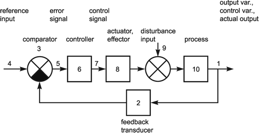
Fig. 8.1 Schematic diagram of a negative feedback control system
Apart from the actuator, an external disturbance, such as light from a suddenly switched on source, may also affect the output variable. The influence of this disturbance input (9) is assumed to be additive, as shown in Figure 8.1. (Disturbances may, of course, occur at any other point in the feedback system, although this will not be discussed here at this stage; but see Chapter 8.6 .)
Actuator and disturbance input thus together influence the actual output variable. In our example this influence produces a change in the output value with practically no delay, because of the high speed of light. In other systems, such as in the control of leg position, the output variable (because of the leg's inertia and frictional forces) does not change within the same course of time as the force generated by a muscle and a disturbance input. These properties of the system (here inertia and friction) are summarized in an element known as process (10). In the example of the pupil control system, the process thus corresponds to a constant (zeroth order system) and can therefore be neglected in this case.
Why is it that a feedback system can reduce the influence of a disturbance input, whereas this is not possible with an open loop control? The crucial difference lies in the feedback element of the former. Via the feedback loop, which contains the feedback transducer, information relating to changes in the actual output are registered. The error signal provided by the comparator allows determination of whether these changes are being caused by a change in the reference input or by the occurrence of a disturbance input. If the reference input has remained constant, the change has to be attributed to a disturbance input. In this case, an error signal different to zero is obtained. This constitutes a command to the controller, which in turn 'tells' the actuator to counteract the disturbance. An increase in the actual output by a disturbance has to be offset by a reduction from the actuator. If a disturbance input is introduced that reduces the value of the output quantity, a positive influence of the actuator on the output quantity is obtained. Because of this sign reversal in a feedback control system, one speaks of negative feedback. It should however be stressed that, as explained in the latter case, such a negative feedback can also produce positive effects, depending on the sign of the error signal.
If the reference input continues to exhibit the same fixed value, this is known as a homeostasis. If it is variable, however, this is called a servomechanism. According to the filter properties with which the controller (6) is endowed, we can distinguish between three different types, whose most important properties will be listed here, but explained later ( Chapter 8.5 ). (This description is, however, only valid when the feedback loop contains a proportional term. In Chapter 8.5, additional possibilities are also discussed.) If (6) is a proportional term with or without delay, i. e., a low-pass filter or a constant, we speak of a proportional controller (P-controller). The most important property of a system containing a P-controller is the fact that, even in the stationary case, in reaction to a step-like disturbance input, an error signal unequal to zero will always persist and its value is proportional to that of the disturbance value. If (6) consists of an integrator, an integral controller (I-controller) is obtained. Unlike a P-controller, in a system with an I-controller the error will be zero in the stationary case. If (6) is a high-pass filter, we speak of a differential controller (D-controller). A feedback system with a D-controller shows a brief response to a step-like disturbance input, which however quickly descends to zero. The compensatory effect of this system is therefore only of short duration and the stationary error signal is equal to the disturbance input. The term adaptive controller is used if the properties of the controller are not fixed but can be influenced by external signals.
Negative feedback is required to compensate for the effects of a disturbance input. Three types of controllers are distinguished: an I-controller fully compensates the effect of a constant disturbance input. By a P-controller, the effect of such disturbance input is compensated, but for a proportional value. A D-controller shows a compensatory effect only for a short time.
The basic quantitative properties of a feedback system will be explained by using the simplified system, shown in Figure 8.2. The various elements mentioned in Figure 8.1 have been combined here to form just two elements of the zeroth order endowed with the amplification factors k1 and k2, i. e., two proportional terms without delay. We are thus dealing with a proportional controller. With the aid of auxiliary variables h0, h1 and h2, as shown in Figure 8.2, the following relations can be formulated for this system:
This results in
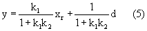
With the abbreviations C1 = k1/(1+k1k2) and C2 = 1/(1+k1k2) we obtain
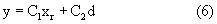
This equation illustrates how output quantity y depends on reference input xr and disturbance input d. If the disturbance input d = 0, the equation can be simplified to y = C1 xr. The actual output is thus proportional (not equal) to the reference input xr. Equation (5) also shows that, in the case of a P-controller, the actual output is proportional to the disturbance input. This accounts for the property, as mentioned, of a system with P-controller, namely, that the effect of a constant disturbance input can never be turned into zero, but, weighted with the factor C2, will always contribute to the output value. With a reference input xr = 0, and a disturbance input d ≠ 0 the deviation from the originally desired value y = 0 no longer takes the value d, but still retains the value C2 d.
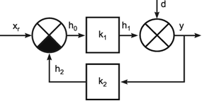
Fig. 8.2 A simplified version of a feedback controller with static elements. xr reference input, d disturbance input, y control variable, h0, h1, h2 auxiliary variables, k1, k2 constant amplification factors
The size of this deviation depends on the choice of constants k1 and k2. The effect of the feedback system is large when C2 is small, that is, when k1 and k2 are large. In order not to make the amplification factor of the feedback system, C1, too small, k1 should be large, and k2 small. Since both goals cannot be realized at the same time, a compromise is inevitable. As will be shown later, there are additional conditions that have to be fulfilled, since otherwise the system may become unstable (see Chapter 8.6 ). The following can be stated with respect to the possible values of constants C1 and C2: Both quantities are always larger than zero. Since k1 and k2, too, are always larger than zero, we get C2 < 1. Since C1 = k1C2, C1 is smaller than 1 if k1 < 1. If k1 is sufficiently large, C1 may also be > 1, but only if k1 remains < 1. If k2 ≥ 1, C1 will always be smaller than 1.
If one wants to investigate such a feedback system, in principle the values of the constants k1 and k2 are obtained in the following way. In the first experiment, the disturbance input d is kept constant, while the reference input xr is varied. The slope of the line obtained when plotting y versus xr provides the constant C1. Conversely, if the reference input xr is kept constant, and the disturbance input varied, the slope C2 is obtained when plotting y versus d. Values k1 and k2 can be calculated from C1 and C2, after which the feedback system will have been completely described.
If the feedback control system is not endowed with simple proportional terms, but with linear filters exhibiting a dynamic behavior, the approach just outlined is still applicable for the static part of the response. k1 and k2 would then be the static amplification factors. If one is also interested in the dynamic part of the behavior of the feedback system, however, calculations will be more difficult because, in equations (1) and (2), convolution integrals will now occur with the weighting functions g1(t) and g2(t) (Fig. 8.3), as follows:

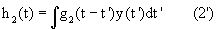


Equations (1')-(4') cannot be solved unless special mathematical methods are used. These are mentioned in Appendix I .
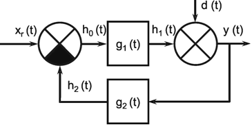
Fig. 8.3 A simplified version of a feedback controller with dynamic elements. xr(t) reference input, d(t) disturbance input, y(t) control variable, h0 (t), h1(t), h2(t) auxiliary variables, g1(t), g2(t) weighting functions, describing the dynamic properties of the systems in the feedforward and the feedback channel, respectively
It will be briefly noted here how the input-output relations of these feedback systems can be determined for the static case, if nonlinearities occur. For this purpose, a static nonlinear characteristic will be assumed instead of the constant k1. Equation (1) then changes from h1 = k1 h0 to
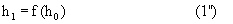
Function f(h0) here defines the nonlinear characteristic. By combining equations (2), (3), and (4), we obtain a new set of equations:


If it is possible to represent f(ho) as a unified formula, one can try to solve these equations arithmetically. Otherwise a graphic solution is possible. To this end, functions (1 ") and (7) are represented in a coordinate system using ho as independent and h1 as dependent variable (see Fig. 8.4). The intersections of the lines are the points whose coordinates fulfill the equations, that is, they are the solutions of the equation system. Figure 8.4 shows this for the example of f(h0), being a nonlinear characteristic endowed with a threshold and saturation. The corresponding output value y can be obtained from the coordinates of the intersection, with reference input xr and disturbance input d taking known values. If xr or d are changed, a new value for y is obtained by a parallel shift of the line, accordingly. Depending on the form of the characteristic, several intersections are possible, and several output values y may result for the same input values xr and d. This occurs, for instance, when the nonlinear characteristic is in the form of a hysteresis. Similarly, if, in the feedback system, a static nonlinear characteristic is present instead of constant k2, equation (7) will become a nonlinear function. In this case, too, the solutions may be obtained by the graphic method as discussed.
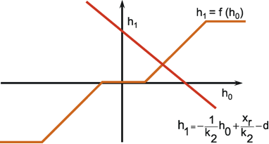
Fig. 8.4 Graphical solution of input-output relation of a negative feedback system with a nonlinear characteristic f(h0) in the feedforward channel. Equation (7) is graphically illustrated by the red line. Its position depends on the values of the parameters xr and d. Changing these parameters results in a parallel shift of this line. As an example, the nonlinear characteristic h1 = f(h0) is endowed with threshold and saturation (yellow lines). For given values xr and d the intersection of both lines indicates the resulting variable h1. Equation(4) (y = h1+d) aIlows determination of the value of the actual output
When the static properties of a feedback system are considered, a simple calculation is possible (see e. g. equations (1) -(5). This can also be extended to systems with nonlinear static characteristics. For the dynamic case, more sophisticated methods (e. g., Laplace transformation) have to be used.
A feedback system can be described as a system endowed with two input values, reference input xr and disturbance inputs d, as well as an output, actual output y (Fig. 8.5a). If this "black box" is filled with a simple feedback system, as shown in Figure 8.2, the problem appears somewhat complicated at first (Fig. 8.5b). If, on the other hand, the equation (6) is taken into account, the feedback system can be simplified (Fig. 8.5c). As discussed, the values of C1 and C2 - and, therefore, the values of k1 and k2 - can be determined easily. Frequently, however, the problem in studying biological feedback systems is posed by the fact that reference input xr is not accessible by experimentation. But in spite of this limitation, there are two possible ways of studying a feedback system, at least partially, in this case.
Fig. 8.5 (a) The negative feedback system as a black box. (b) A view inside the black box. (c) Rearrangement of the internal structure shows an equivalent feedforward system. xr reference input, d disturbance input, y control variable, or actual output, C1, C2, k1, k2 constant amplification factors
One possibility is to examine the relation between disturbance input and actual output. In Figure 8.5 c, this corresponds to the determination of value C2. The disturbance input is used as input, the actual output as output of the system. In these measurements, it has to be presupposed that the reference input remains constant during the investigation. The second way is a study of the open loop feedback system. A feedback system is opened, if it has been possible in some way to ensure that the value measured by the feedback transducer is no longer influenced by the actuator. This can be done by an interruption of the feedback loop between output variable and feedback transducer, as illustrated schematically in Figure 8.7. The input of the feedback transducer is then used as a new input xol of the open loop system. In this way, the problem has been reduced to the simpler task of the study of a system without feedback. In order to avoid confusion between the open loop feedback system and open loop control mentioned earlier, it is better to speak of the "opened" loop in the former case. However, as this is not usual in the literature, we also will speak of the open loop system where we mean the opened feedback system.
A feedback system can be opened in different ways. If it is possible, the simplest way is to open the feedback loop mechanically. This will be explained for the example already used in Figure 7.1. In the legs of many insects there is a feedback control system which controls the position of a leg joint, the joint connecting femur and tibia. The position of this joint is measured by a sense organ, the femoral chordotonal organ which is fixed at one end to the skeleton of the femur and at the other to the skeleton of the tibia by means of an apodeme, thus spanning the joint (Fig. 8.6). Because of this morphological arrangement, the more this sense organ is stretched, the more the femur-tibia joint is flexed. The reflex loop is closed such that by a dilatation of the sense organ-corresponding to a flexion of the joint-the extensor muscle is activated in order to oppose the flexion, whereas after a shortening of the sense organ the antagonistic flexor muscle becomes active. In this feedback system the loop can be opened mechanically by cutting the apodeme of the sense organ. The input function can then be applied by experimentally moving the apodeme and thereby stimulating the sense organ. The activation of the muscles can no longer influence the value measured by the sense organ, thus the loop is opened. The two following examples show that eventually more elegant methods can also be used. For example, opening the pupil feedback system is very easy. The input of the feedback transducer is the illumination of the retina, subject to change by external illumination; the actual output is the pupil area. There is a difficulty when investigating the system in using a step function as input function, i. e., by suddenly switching on an additional light source. In this case the illumination of the retina is not changed in a step-like way. Due to the effect of the feedback system, the illumination is reduced again by the contraction of the pupil area. (By using an impulse function, this problem does not occur, provided the impulse is sufficiently short.) In the experiment, the problem can be avoided by using a light beam projected onto the retina which is narrower than the smallest possible pupil diameter (see Box 3 ). In this way, the experimentally generated illumination can no longer be influenced by the impact of the feedback system. The feedback system is thus opened.
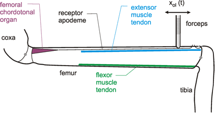
Fig. 8.6 Morphological basis of a resistance reflex in the leg of an insect. The angle between femur and tibia is monitored by the femoral chordotonal organ, which is mechanically connected to the tibia by a long receptor apodeme. By cutting this apodeme, the loop can be opened and the apodeme can be moved experimentally using a forceps and thus the xol input can be applied ( Bässler 1983 )
A further example of the opening of a feedback system is used in the study of system which controls the position of a leg joint ( Bässler 1983 ). The joint is bent by the experimenter with great force, and the opposing force exerted by the system is measured at the same time. The bending force must be sufficiently great to prevent the counterforce developed by the feedback system from influencing the form of the bending to any measurable extent. In this example, too, the feedback system is thus opened. The advantage of both methods lies primarily in the fact that no surgical intervention with a potentially modifying effect are required, as is possible in the first example.
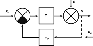
Fig. 8.7 A negative feedback system as shown in Fig. 8.3, illustrating the input xol in the case of an opened loop. xr reference input, d disturbance input, y control variable. F1 and F2 represent the filter in the feedforward channel and the feedback channel, respectively
In the example shown in Figure 8.7, for the static case we obtain y = - k1k2xol, if k1 and k2 constitute the static amplification factors of the filters F1 and F2. This shows, though, that both methods, i. e., the study of the open feedback system (input xol, output y) and the study of the impact of the disturbance input on the closed loop (input d, output y), give information only on the product k1k2. The individual amplification factors of filters F1 and F2 can thus not be calculated separately. This means that even using both methods does not show the location where the reference input enters the system. Therefore, after these investigations, little or nothing can be said as to how the feedback system responds to a change in the reference input. This is only possible in such cases where the reference input can be manipulated experimentally. An example is pointing movements in humans. In this case, the subject can be shown where to point. If the subject is prepared to cooperate, arbitrary functions can be chosen for the reference input.
There are three possible ways to investigate a feedback controller, namely to experimentally change the reference input, the disturbance input, or, by opening the loop, by investigation of the opened loop response. Complete information about the system is only available if the first and at least one of the two latter methods can be applied.
The problem mentioned in the last paragraph occurs independently of whether systems of the zeroth, first or higher orders are involved, that is, no further information can be obtained from the dynamic part of the responses. In the following, some examples will illustrate the behavior of all three controller types, mentioned above, namely the P-, D-, and 1-controllers. To this end, the xr, d, and xol responses of the feedback system shown in Figure 8.7 are compared, while different filters are substituted for F1 and F2.
According to equations (5) and (5'), we get the factors C1 and C2 according to C1 = k1/(1 + k1k2) and C2 = 1 /(1 + k1k2). In the case of proportional elements, k1 and k2 denote the static amplification factors of filters F1 and F2. If a high-pass filter is present, the maximum dynamic amplification factor kd ( Chapter 5.3 ) has to replace the static amplification factor (which is always zero for a high-pass filter). The static amplification factor of a high-pass filter is used only in calculating the static opened loop response, i. e., using xol as input (Fig. 8.7). In the case of an integrator, the integration time constant τi has to be taken into account (see below). In the examples chosen here (Fig. 8.8), we assume k1 = 0.5, and k2 = 1.This means that C1 = 0.33, and C2 = 0.66. The integration time constant is assumed to be τi = 1 for Figure 8.8e and τi = 0.5 for Figure 8.8f. To show the dynamic properties of six different negative feedback system, the temporal change of the actual output y (see Figure 8.7) is presented, when a unit step function is given to the reference input xr, the disturbance input d, or the input of the opened loop xol,. The response to the disturbance input is shown by dotted lines.
a) Let filter F1 be a 1st order low-pass filter with the time constant τ and the static amplification factor k1, and filter F2 be a constant (a zeroth order system) with amplification factor k2. The step response of the open loop (input xol) is that of a low-pass filter endowed with the static amplification factor k1k2 and the time constant τol = τ (Fig. 8.8a, xol). If, in the case of a closed loop, the disturbance input d is used as input, a step response is obtained which first ascends to value 1, then, with the time constant τcl = C2τ (cl = closed loop), descends to the static value C2 (Fig. 8.8a, dashed line). As C2 is always smaller than 1 (see Chapter 8.3 ), the time constant of the closed loop is smaller than that of the open loop system. Here, the influence of the disturbance input is diminished from value 1 to value C2 (C2 < 1), but not to zero. It is typical of a P-controller (F1 is a proportional term) that, in the case of a step-like disturbance input, a continuous error persists. The response of the closed loop system to a step-like change in the reference input xr corresponds to that of a low-pass filter endowed with the time constant τcl = C2 τ and the static amplification factor C1 (Fig. 8.8a, xr). The time constant of the closed loop thus also depends on amplification factors k1 and k2.
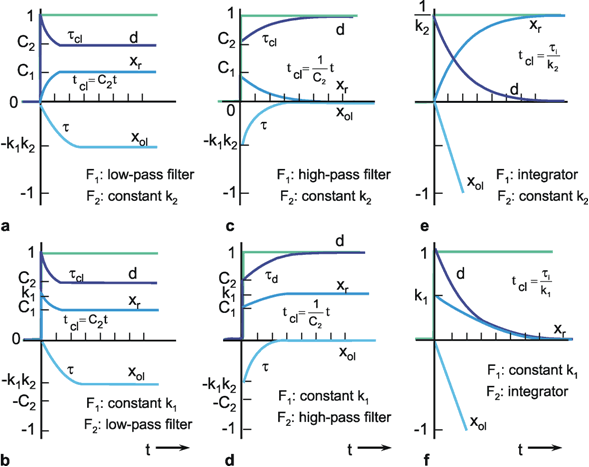
Fig. 8.8 The step responses of the actual output y when a unit step (green lines) is given to the reference input xr (blue lines), the disturbance input d (dark blue lines), or the input of the opened loop, xol (light blue lines). Different combinations of filters F1 and F2 (see Fig. 8.7) are used (constants, low-pass filter, high-pass filter, and integrator, as mentioned). The meaning of the different parameters is explained in the text. The differences between the time constants of the open and the closed loop, τ and τ cl,, are graphically enlarged for the sake of clarity.
b) If the two filters are interchanged such that F1 now represents a constant amplification factor k1, and F2 a low-pass filter endowed with the time constant τ and the static amplification factor k2, we are still dealing with a P-controller. The response of the open loop system agrees with that of the previous example as, in linear systems, the sequence of the series connection is irrelevant (8.8b, xol). Also the response of the closed loop to a step-like disturbance input d exhibits the same course as in the first example (Fig. 8.8b, dotted line). Both feedback systems thus can not be distinguished in this respect. On the other hand, they respond differently to a step-wise change in the reference input xr as the step response (Fig.8.8b, xr) shows. This response initially jumps to value k1 and then, with time constant τcl = C2 τ, descends to the value C1. The occurrence of this response can be explained as follows: First, the step weighted with factor k1 fully affects the output. Only then does an inhibiting influence occur via the feedback loop, whose time course is determined by the "inert" properties of the low-pass filter.
c) Figure 8.8c shows the case of a system with D-controller. Filter F1 is a 1st order high-pass filter with time constant τ, the maximum dynamic amplification factor kd = k1, and the static amplification factor ks = 0. Filter F2 is formed by the constant k2 (zeroth order system). The step response of the open loop is that of a high-pass filter of time constant τ and the maximum dynamic amplification factor k1 k2 (Fig. 8.8c, xol). In studying the response to a step-like disturbance input in the case of a closed loop, we note that, immediately after the beginning of the step, the former decrease from value 1 to value C2 (Fig. 8.8c, dotted line). In the course of time, though, the effect of the feedback diminishes. With the time constant τcl = τ/C2 (i. e., τcl > 1), the step response ascends to the final value 1. Is should be noted, however, that by using a "realistic high-pass filter," that is, a band-pass filter, the disturbance cannot be turned down immediately. Rather, the maximum feedback effect occurs only a little later, as it depends on the upper corner frequency of the band-pass filter. In principle, it can be said that the feedback effect of a system with D-controller occurs very quickly, but also that it descends to zero after some time, so that the disturbance input can then exert its influence without hindrance. A further property of the D-controller is mentioned in Chapter 8.6 .
The response of the closed loop to a step-like change in the reference input xr corresponds to that of a high-pass filter endowed with time constant τcl = τ/C2 and the maximum dynamic amplification factor C1 (Fig. 8.8c, xr). With this feedback system, it is thus not possible to retain an actual output that is constant and derivates from zero over a prolonged period of time. If this process which takes place in the closed loop is simplified by mentally separating it into two successive simple processes, the result can be explained in qualitative terms as follows: The high-pass response to the input function is subtracted from the input function via the feedback loop. This new function, which comes close to the step response of a low-pass filter, now constitutes the new input function for high-pass filter F1. On account of the prolonged ascent of this function, the response of the high-pass filter is also endowed with a greater time constant τcl.
d) If filters F1 and F2 are interchanged again such that F1 be a constant k1, F2 a 1st order high-pass filter endowed with the time constant τ and the maximum dynamic amplification factor k2, the same responses are obtained for the input quantities xol and d, as in example c) (Fig. 8.8d). Again, after these investigations, it is not possible to make a statement concerning the behavior of the feedback system in response to changes in the reference input. In this case, the step response to a change in the reference input jumps initially to value C1 and then, with the time constant τcl = τ/C2, ascends to the final value k1 (Fig. 8.8d, xr).
e) In the next example, an integrator with the a time constant τi (see Chapter 4.8 ) is used as filter F1, and a constant k2 as filter F2. The step response of the open loop is a line descending with the slope –k2/τi (Fig. 8.8e, xol). The step response to a step-like disturbance input d initially jumps to 1, that is, the disturbance input fully affects the actual output. Subsequently, though, the latter decreases with the time constant τcl = τi/k2 to zero, so that the effect of the disturbance input is fully compensated in the case of an I-controller (Fig. 8.8e, dotted line). This happens because the output value of the integrator increases as long as the error signal is different from zero. If the error signal, and hence the input value of the integrator, equals zero, the integrator retains the acquired output value. The response to a step-like change in the reference input corresponds to a step response of a low-pass filter endowed with time constant τcl = τi /k2 and the static amplification factor 1/k2 (Fig. 8.8e, xr).
f) In interchanging the two types of filters - F1 is now a constant k1 and F2 an integrator of the integration time constant τi - one again obtains the same responses as in e) (Fig. 8. 8f), apart from the difference between k1 and k2, for open loop systems and for the change in the disturbance input. If the reference input of the closed loop is changed, however, a completely different step response is obtained. It corresponds to the step response of a high-pass filter of the time constant τcl = τi/k1 and the maximum dynamic amplification factor k1(Fig. 8.8f, xr). Again, in this example as in that of c), no constant actual output values that are different from zero can be adopted either.
Examples e) and f) show an alternative way of constructing a low-pass and a high-pass filter, respectively, using a feedback system with integrator. These circuits provide the basis for the simulation of those filters shown in Appendix II .
In accordance with the definition given in Chapter 8.2 , the feedback systems shown in Figure 8.8d and 8.8f are endowed with P-controllers, since in both cases filters F1 are proportional terms. However, the rule that, with a P-controller at a constant disturbance input, a continuous error signal persists - which is smaller, though, than the effect of the disturbance input in itself - does not apply to these two cases. It only applies if no terms other than proportional ones occur in the feedback branch. For biological systems, this cannot be automatically assumed, however. The examples mentioned above should therefore also serve to illustrate other possibilities. A possible process (Fig. 8.1) was not considered here for reasons of clarity. An example taking the process into account will be described below.
It has already been pointed out that, in the case of a D-controller (Fig. 8.8c), the compensation of the effect of a disturbance input is much more rapid than with a P-controller (Fig. 8.8 a, b). The reason is that a P-controller is maximally effective only in the static range, whereas a D-controller operates maximally right from the start of the ascent of the disturbance input, since the value of the first derivation is highest at this stage. A major disadvantage of a D-controller is that the static effect is zero, i. e., that the disturbance input exerts its full influence in the static case. In technical systems, a parallel connection of P- and D-elements is frequently used to eliminate this disadvantage. The result is a P-D-controller. Compared to the P-, D-, and P-D-controllers, the I-controller is endowed with the property of changing its controlled variable until the error signal equals zero, that is, until the disturbance input is fully compensated. The disadvantage of the I-controller lies in the fact that it operates even more slowly than a P-controller. For this reason, P-I- or P-I-D-controllers, produced by the corresponding parallel connections, are used in technology, and probably in biology, too, thus combining the advantages of all types of controllers.
Although I-controllers appear more useful than P-controllers, since for the latter the disturbance input is only partially compensated, P-controllers are the rule in biological systems. How could this be explained? Actually, the use of a P-controller makes particular sense, if a specific variable is controlled by several, e. g., two, feedback systems rather than just one such system, as is frequently the case in biological systems. A familiar example is position control in fish. v. Holst showed that the position of the vertical body axis is controlled via visual pathways ("dorsal light response") as well as the otolith organs (v. Holst 1950 a , b ). If the reference inputs of the two feedback systems do not absolutely agree, the control for outputs of both loops operate consistently against each other. When P-controllers are involved, both controller outputs take constant values which are proportional to the (usually small) deviation. In the case of I-controllers, however, the output values of the two controllers, which are operating against each other, would ascend to their maximally possible values. In this case, the use of I-controllers would obviously be uneconomical.
To summarize, we can say that, in principle, there is no problem in investigating the response of a biological feedback system to changes in the disturbance input. This is sufficient for a homeostatic feedback system. If a servomechanism is involved, however, the behavior of the feedback system in response to changes in the reference input would be of interest. As long as the reference input is not accessible, though, only very indirect conclusions can be drawn from these investigations or the study of the open loop feedback system.
When, however, we are interested in the transfer properties of the controller and of the process, for instance in the above mentioned example of bending the joint of a leg, the situation can be described by Figure 8.9. k, is the amplification factor of the controller and k3 is that of the process, i. e., the elasticity of the muscles. k3 describes the transformation of force f produced by the muscles into position p, k, correspondingly the transformation from position (error signal) into force. Without loss of generality we can assume the reference input x, to be zero. Then, we have the equations f = k1k2pol under open loop conditions and p = k3/(1 + k1k2k3) d = kcl d under closed loop conditions, i. e., when we load the leg and measure the position obtained under disturbances. Thus, k1 and kcl are measured and k3 can then be calculated.
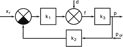
Fig. 8.9 A negative feedback system for position control including a process (k3). k1 and k2 describe the gain of the controller and the feedback transducer, respectively, d disturbance input, f force developed by the controller (+ actuator which is not shown here) and the disturbance input, p position output, pol position input when the loop is experimentally opened
However, as a general comment it should be remembered that all these considerations, regarding comparison between open loop and closed loop investigation, hold only on condition that the system always remains the same, regardless of the kind of investigation. This is not always the case, as results of Schöner (1991) , investigating the posture control in humans, and results of Heisenberg and Wolf (1988) , considering the orientation response of Drosophila, have shown. The latter work shows an interesting, nonlinear solution of the control problem.
Several examples showing the dynamic properties of different feedback controllers are shown in Figure 8.8. In some cases, the behavior of the complete system corresponds to that of a low-pass filter or a high-pass filter. The properties of P-, I-, and D-controllers can be combined to obtain the advantages of the different elements. In biology I-controllers are less often used than P-controllers, because the former cannot be combined with other feedback system to control the same actual output value.
Earlier we found that, on the basis of investigations of the opened feedback system, little can be said about the properties of the closed loop regarding its behavior in response to changes in the reference input. But there is one important property about which a statement can be made after the study of the open loop. This concerns the question of the stability of a feedback control system. Such a system is unstable, if the value of the output variable grows infinitely in response to an impulse- or step-like change in the input variable (reference input or disturbance input). Usually, the output variable of an unstable feedback system exhibits oscillations of increasing amplitude. In reality, however, the amplitude is always limited by an nonlinearity. In some cases, such oscillations may even be desirable (e.g., to generate a circadian rhythm). But in a feedback system constructed to keep a variable constant, such oscillations should be avoided.
The origin of these oscillations can be illustrated as follows: assume that any kind of input function is given to an input, for example the disturbance input. According to the Fourier decomposition, this input function can be considered to consist of the sum of several sine functions. When these sine functions pass the sign reversal at the comparator, this corresponds mathematically to a phase shift of 180°. Further phase shifts may be caused by the presence of a higher order low-pass filter or a pure time delay. If one takes account of that sine oscillation which, by passing the loop, receives a phase shift of 180° in this way, together with the effect of the sign reversal, an overall phase shift of 360° will result for this frequency. This means that the same sine function (except for an amplification factor) is added to the sine function of the input variable. Since this is repeated for each cycle, an oscillation results that keeps building up, and whose amplitude increases infinitely under certain conditions.
With the aid of the so-called Nyquist criterion, it is possible to decide, on the basis of the properties of the open loop system (i.e., the opened feedback system) whether the closed loop system is stable or unstable. The Nyquist criterion can be applied to the Bode plot of the open loop response as follows. (These data are applicable only if the impulse response of the open loop, that is, its weighting function, does not grow infinitely with increasing time. For the application of the Nyquist criterion in other cases, the reader is referred to the literature ( DiStefano et al. 1967 , Varju 1977 )). First, the Bode plot of the open loop feedback system will be studied with a view to identifying critical situations. A total of eight different situations (S1-4, I1-4) are possible:
S1: The amplitude frequency plot crosses the amplification-1 -linie with negative slope.
The phase shift at this frequency comprises 0°> ϕ > -180°.
S2: The amplitude frequency plot crosses the amplification- 1-line with positive slope. The phase shift at this frequency comprises 0° < ϕ < 180°.
S3: The phase frequency plot crosses the -180°-line with positive slope. The amplification factor at this frequency is > 1.
S4: The phase frequency plot crosses the -180°-line with negative slope. The amplification factor at this frequency is < 1.
I1: The amplitude frequency plot crosses the amplification-1 -line with positive slope. The phase shift at this frequency comprises 0°≥ ϕ ≥ -180°.
I2: The amplitude frequency plot crosses the amplification- 1-line with negative slope. The phase shift at this frequency comprises 0°≤ ϕ ≤ -180°.
I3: The phase frequency plot crosses the -180°-line with negative slope. The amplification factor at this frequency is ≥ 1.
I4: The phase frequency plot crosses the -180°-line with positive slope. The amplification factor at this frequency is ≤ 1.
With the aid of these situations, the Bode plot of the open loop system is characterized in the following way. First, these critical situations have to be identified and noted in order of appearance beginning with the low frequencies. Figure 8.10 shows the Bode plots of three different systems. All of them are endowed with the same amplitude frequency plot, i. e., they differ only in terms of their phase frequency plot. The following critical situations are obtained for these three Bode plots (1): S1, S4; (2): I3,I2; (3): I3, S3, S1, S4. If in this sequence, two situations with the same figure are placed next to each other (as in (3) for I3, S3), both have to be canceled. If this result in two further situations with the same figure becoming neighbors, they, too, have to be eliminated. This procedure is continued until no further eliminations are possible, i. e., no situations with the same figure occur next to each other. Then only situations should occur belonging to either the S class or to the I class. In the first case (S), the closed system is stable, in the second case (I), it is unstable.
The application of the Nyquist criterion to the Bode plot of the open loop feedback system can be considerably simplified, if in the entire Bode plot no more than two of these critical situations are present, as is usually the case. (In Figure 8.10, this is true for systems (1) and (2).) For this purpose, we will introduce the concept of phase margin ϕm. If, at the frequency where the amplitude frequency plot crosses the amplification-1-line, the open loop system is endowed with the phase shift ϕ, then the phase margin can be calculated by ϕm = 180° + ϕ (Fig. 8.10 (1)). The phase margin thus represents the difference between -180° and the phase shift at the frequency considered. (ϕ m is defined only between - 180° < ϕ m < 180°.) With respect to this simple case, it could be said therefore that the closed system is stable, if ϕ m > 0, and that it is unstable, if ϕ m <0.The frequency at which the open loop system shows a phase shift of -180° is known as critical frequency. If a feedback system is still in a stable range, but close to the limit of stability, this can be observed in the behavior of the system. The smaller the phase margin, the faster is the response to a step function, but the more prolonged, too, are the transient oscillations to the stationary value. The closer the system is to the limit of stability, the worse the "quality of stability" thus tends to become. In technical systems, the rule concerning a reasonable quality of stability states that the phase margin should be 30° to 60° at least. In the unstable case, the feedback system carries out oscillations with that frequency at which the phase frequency plot intersects with the - 180° line, i. e., the critical frequency.
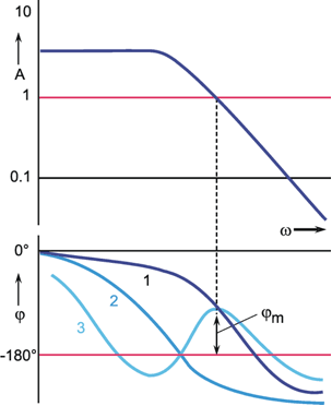
Fig. 8.10 The Bode plots of the open loop system of three different feedback controllers. The amplitude frequency plot is assumed to be the same in all three cases. The form of the different phase frequency plots (1-3) shows that the feedback controllers with the phase frequency plots (1, dark blue line) and (3, light blue line) are stable, whereas the plot no. (2, blue line) belongs to an unstable controller, because in this case the phase margin ϕm is negative
When we look at the open loop Bode plot of a stable system ((1) in Figure 8.10), we recognize that a stable system can be made unstable by increasing its amplification factors. Leaving the phase frequency plot unchanged, the intersection of the amplitude frequency plot with the amplification-1-line is shifted to higher frequencies. Another possibility would be to increase the phase shift, e. g., by increasing the dead time of the system, leaving the amplitude frequency plot unchanged. This phenomenon is observed in connection with the impact of alcohol on the central nervous system. Everyone is familiar with the resultant oscillations. Two methods for artificially raising the amplification factor for the pupil control system are described in Box 3 . Thereby, the system can be stimulated to show continuous oscillations of the pupil diameter at a frequency of about 1-2 Hz.
It should be pointed out at this stage that any assumption concerning the inference of the closed loop from the open loop system is meaningful only, if the actual, (i. e., dimensionless) amplification factor of the open loop system can be given. For this, the input and output value has to be measured using the same dimension, or has at least to be converted into the same dimension. However, as was pointed out in Chapter 2.3 , this is not always possible in the study of biological systems.
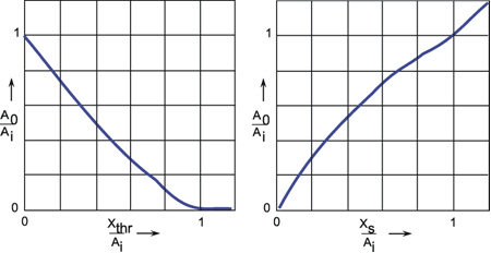
Fig. 8.11 Gain factors for the fundamental wave for (a) a nonlinear characteristic with threshold value xthr (see Fig. 5.10) and (b) a nonlinear characteristic with saturation value xs (see Fig. 5.9). A1 input amplitude, Ao output amplitude (after Oppelt 1972 )
Stability of nonlinear feedback systems. The Nyquist criterion is strictly applicable to linear systems only. The calculation of the static behavior of a feedback system endowed with nonlinear static characteristics has been dealt with in Chapter 8.3 . But the question of whether such a feedback system is at all stable, that is, whether a static behavior exists at all, was not addressed. In the following, we will therefore answer the question of when such a nonlinear feedback system is unstable. An approximate solution to this problem is possible with the following assumption: The filters occurring in the total system, apart from the nonlinear static characteristic, are endowed with low-pass properties that have the effect that the harmonics generated in the sine response by the nonlinear characteristic are considerably weakened after having passed the closed loop. This leaves only the fundamental wave as an approximation to be considered. The relation of the maximum amplitude A0 of the fundamental wave at the output to the maximum amplitude Ai of the sine oscillation at the input can be defined as the amplification factor of the nonlinear characteristic. This amplification factor depends both on the size of the input amplitude and on the position of the point of operation. In Figure 8.11 a, b, these amplification factors are given for the case of a characteristic with a threshold (Fig. 5.10) and a characteristic with saturation (Fig. 5.9) for different threshold (xthr ) and saturation values (xs) and various input amplitudes Ai. The slope of the linear parts of the characteristics is assumed to be 1, and the origin of coordinates always to be the point of operation.
If these amplification factors are introduced for the nonlinear static characteristic of the feedback system, the system can then be considered linear under the conditions mentioned earlier. The amplitude frequency plot of the opened loop is obtained by multiplying the amplitude frequency plot of the linear feedback system with this amplification factor. The Nyquist criterion may be applied to this. This shows that, with respect to a nonlinear feedback system, one can no longer speak of the system as such being stable or unstable. Rather, the stability of a nonlinear feedback system may depend on the range of operation involved. If nonlinear dynamic characteristics are present, the phase shifts produced by the nonlinearity may also be considered accordingly; but this will not be further discussed here (see e. g., Oppelt 1972 ).
Rather than oscillations of an infinitely large output amplitude, a feedback system that is unstable will, due to a characteristic with saturation, always produce only limited maximum amplitudes in a real situation. One example, discussed earlier, is the pupil control system. By an artificial increase in the amplification, this feedback system can be rendered unstable and it responds by continuous oscillations of a constant amplitude and frequency. Such oscillations are also known as limit cycles. Depending on the relative position of nonlinearity and low-pass elements in the loop, these limit cycles may be considerably distorted by the nonlinearity, as shown in Figure 5.9, or may produce nearly sine-shaped oscillations of small amplitude (see Box 3 ).
An example of a feedback system in which limit cycles almost always occur is the so-called two-point controller. This is a nonlinear controller which has the characteristic of a relay, i. e., there is an input value above which the control signal always takes position 1 (e. g., "on"), and below which it takes position 2 (e. g., "off") (Fig. 5.12). The temperature control of a refrigerator, for instance, operates according to this principle. If a critical temperature is exceeded, the cooling aggregate is switched on. If, after some time, the critical temperature falls below a certain threshold, the motor is switched off and the refrigerator warms up again. Its actual temperature thus oscillates regularly around a critical temperature. The relay characteristic may be considered formally as a characteristic with saturation and, on account of the vertical slope, with an infinitely high amplification. In view of the high amplification and the time delay present in the system, this is unstable. Due to the saturation, however, no infinitely increasing oscillations, but limit cycles of a constant amplitude are obtained. The presence of a hysteresis-like characteristic, e. g., a real relay (Fig. 5.16), influences the occurrence of limit cycles. The time required to get from one switch point of the relay to the next has an effect that is analogous to a dead time and thus to a time delay.
A system with positive feedback can be stable if the feedback channel contains a high-pass filter. In this case the whole system has the same properties as a system consisting of parallel connected high- and low-pass filters (Fig. 4.8a). In Appendix I such a system is used as an example to show how to calculate the dynamic properties.
A negative feedback system may become unstable under certain conditions. These are high gain factors and large phase shifts within the loop. A quantitative criterion to judge the stability of the system is given by the Nyquist criterion which is based on the Bode plot of the open loop system. It can also be applied to nonlinear systems in an approximation. Unstable nonlinear systems can show limit cycle oscillations.
The Pupil Feedback System
It was already described in Chapter 8.4 that the feedback system controlling the pupil diameter can be opened experimentally. This is shown in Figure B3.1 ( Milsum 1966 ). The retina is illuminated by a light beam projected on to it that has a diameter smaller than the smallest pupil diameter. In this way change of pupil diameter does not influence the input function.
The responses the step and impulse input functions produced using this technique are shown in Figure B3.1 a-d. An increase in light intensity leads to a decrease of the pupil diameter. The two values of the pupil area A1 and A2 marked in the figures correspond to static response to low and high input intensity, respectively. The response to an increasing step (Fig. B3.1 a) corresponds qualitatively to that of the system shown in Figure 4.7a, namely a parallel connection of a low-pass filter and a band-pass filter with k > 1. However, reversal of the sign of the input functions does not produce a corresponding sign reversal of the output functions for both the step and the impulse response (Fig. B3.1 c). The comparison between the two impulse responses (Fig. B3.1 b, d) shows no corresponding sign reversal either. This means that the system contains nonlinear elements. How can these results be interpreted? The band-pass response is only found when the input function contains a part with increasing light intensity. Therefore, a simple hypothesis to explain these results is to assume a parallel connection of a low-pass filter and a band-pass filter as in Figure 4.7a, but with a rectifier behind the band-pass filter. Furthermore, there is a pure time delay which causes the dead time T mentioned in the figures.
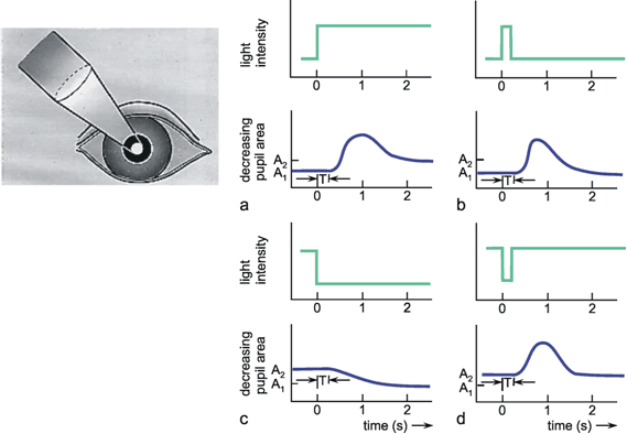
Fig. B 3.1 Changes of the pupil diameter when the central part of the pupils is stimulated by a step function (a), (c), or an impulse function (b), (d). T marks the dead time of the system
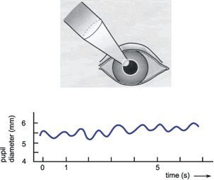
Fig. B3.2 Limit cycle oscillations of the pupil diameter after the gain of the control system has been increased artificially by illumination of the margin of the pupil (after Hassenstein 1966 )
Figure B3.2 shows a way of increasing the gain of the feedback loop ( Hassenstein 1966 ). This can be done by projecting the light beam on the margin of the pupil such that the beam illuminates the retina with full intensity when the pupil is at its maximum diameter, and that the retina receives nearly to light when the pupil is at its smallest diameter. This leads to continuous oscillations at a frequency of about 1-2 Hz (Fig. B3.2). Another very simple and elegant method of raising the amplification factor has been proposed by Hassenstein (1971) . The inner area of the pupil is obscured by a small piece of dark paper held in front of the eye. In this way, the change in the illumination of the retina accompanying a specific dilatation of the pupil diameter, and thus the amplification of the system, is increased. By using paper of an appropriate diameter and chosen according to given lighting conditions, oscillations can be elicited easily. As in humans both eyes are controlled by a common system, the oscillations can be observed by looking at the other, uncovered eye.
In addition to the simple feedback system described above, there is a number of more complicated feedback systems, two examples of which will be discussed to conclude this topic. Figure 8.12 shows a feedback system with feedforward connection of the reference input. The figure shows the two ways in which the reference input operates: it has a controlling effect on the output variable via the comparator, and it directly influences the output variable via a further channel in the form of an open loop (feedforward) control. If constants k1 and k2 are introduced for filters F1 and F2 to calculate the stationary case, the following equations will result, which is analogous to equation (5) in Chapter 8.3 :
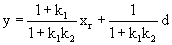
Whereas, in a simple feedback system, the reference input has to take the value

to obtain a particular value y as a output quantity, here is only needs to take the smaller value
 .
.
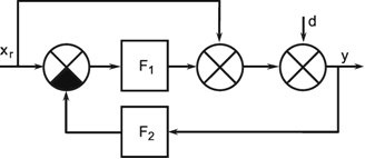
Fig. 8.12 Control system with feedforward connection of reference input. xr(t) reference input, d(t) disturbance input, y(t) control variable, F1 and F2 represent the filter in the feedforward channel and the feedback channel, respectively
The range of input values which the controller has to be able to process is thus smaller in a control system with feedforward of reference input, making it much simpler to construct the controller. This is an interesting aspect especially with regard to systems in neurophysiology, since here the range of operation of a neuron is limited to less than three orders of magnitude (about 1 Hz to 500 Hz of spike frequency). A further advantage of a feedback system with feed-forward of reference input lies in the fact that this can be constructed using a D-controller without the disadvantages described in Chapter 8.5 . On account of the feedforward channel, the output variable receives a sensible input value, even if the output of the D-controller has fallen to zero. One advantage of this circuit lies in the response of the D-controller which is faster than that of the P-controller. Another aspect of this property of the D-controller, which was not discussed in Chapter 8.5 , is that a system that is unstable (due the presence of a dead time, for example) can be made stable by the use of a P-D-controller instead of a simple P-controller. This can be explained by comparing this with Figure 8.10 (2), namely that the phase frequency plot of the open loop is raised by the introduction of a high-pass filter (D-controller), especially at high frequencies, resulting in the fact that the phase frequency plot cuts the -180° line only at higher frequencies (see also Chapter 4.6 ). If the amplification of the high-pass filter is sufficiently small, the total amplification of the open loop may be smaller than 1 at this frequency. The system thus fulfills the conditions of stability.
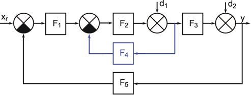
Fig. 8.13 A cascaded feedback system. Xr(t) reference input, d1(t) and d2(t) disturbance inputs, y(t) control variable, F1 to F5 represent unspecified filters
If the structure of the controlled process is more complex, it is sometimes practical to control the value of a variable which represents a precursor of the actual output via a separate feedback system (Fig. 8.13). This is known as a cascaded feedback system. This circuit has the advantage that a disturbance at d, does not have to pass the entire loop (changing the actual output, passing the feedback loop), but is instead controlled beforehand so that the disturbance does not get through to the actual output (for a detailed study of cascaded feedback systems, see DiStefano et al. 1967 ). The cascaded system is a special case of the so-called mashed systems. We speak of a mashed system, if there are points in the circuit from which one can go through the circuit by at least two different routes and return to the same point.
A negative feedback loop with additional feedforward of reference input makes it possible to use a controller with a smaller gain factor. Cascaded feedback controllers can cope better with internal disturbances than can a simple uncascaded control system.
In order to illustrate the properties of feedback systems previously discussed, we will give a highly simplified description of the biological feedback system that controls the position of a joint, for example the elbow, in mammals. The description given will be on a qualitative level, to facilitate comprehension of the subject, and because there is still a number of unanswered questions. For a more detailed study of the underlying structures, the reader is referred to the literature (e. g., Kandel et al. 1991 ). To simplify matters, all antagonistically operating elements, such as muscles, nerves and the various receptors, are subsumed in one unit.
Several mechanisms are involved in the closed-loop control of the position of a joint, the most important being shown (in partly hypothetical form) in Figure 8.14. The anatomical relationships are represented in Figure 8.14a in highly schematic form. Figure 8.14b shows the same system in the form of a circuit diagram. The musculature (actuator) responsible for the position of a joint is innervated by the so-called α-motorneurons. The muscles controlled by the α-fibers produce a force which can shorten the muscle and, in this way, effect a change in the position of the joint. To this end, the mechanical properties (inertia of the joint moved, friction in the joint, elasticity and inertia of the muscles), which represent the process, have to be overcome. The muscle spindles lie parallel with this (the so-called extrafusal) musculature. They consist of a muscular part (the intrafusal musculature), whose state of contraction is controlled by the γ-fibers, and a central, elastic part which contains the muscle spindle receptors. These measure the tension within the muscle spindle. For a specific value of γ-excitation, this tension is proportional to the length of a given muscle spindle and thus to the length of the entire muscle. The response of the muscle spindles to a step-like expansion is of a phasic-tonic kind (Fig. 4.11), i. e., it might, as a first approximation, correspond to a lead-lag system, or, in other words, a parallel connection of a high-pass and a low-pass filter. If a disturbance is introduced into a muscle once its length is fixed (i. e., a particular position of the joint), as symbolized in Figure 8.14a by attaching a weight and in Figure 8.14b by the disturbance input d1, the immediate result is a lengthening of the muscle. Due to the lengthening of the muscle spindle, the Ia-fiber stimulates the α-motorneuron, effecting a contraction of the muscle. The disturbance is counteracted so that we can speak of a feedback system.
Since we observe only stimulating synapses in this system, one obvious question concerns the point at which a reversal of signs occur, which is necessary in a feedback controller. The reversal is tied up with the mechanical arrangement of the muscle spindles, because shortening the muscle also shortens the spindle, which causes a decrease in activity of the sensory fibers. Therefore, the frequency in the la-fiber is reduced when there is an increase in the frequency of the a-motorneuron, in spite of the fact that we have stimulating synapses only.
The γ-fibers also receive inputs from the brain. If the frequency of the γ-fibers is increased via these inputs, the intrafusal musculature of the muscle spindle is shortened. This causes an increase in the frequency of the la-fiber and, because of this, of the α-motorneuron, too. In this way, the length of the muscle (and thus the position of the joint) can be controlled via the γ-motorneuron. The γ-fibers, can therefore be regarded as the transmitters of the reference input. As early as around 1925 to 1927, Wagner interpreted this system as a servomechanism ( Wagner 1960 ). It seems his work then fell into oblivion, and this interpretation surfaced again only in 1953 ( Stein 1974 ).
For some time it has been known that α-motorneurons also receive inputs directly from the brain. Recent studies have shown that, during active voluntary movements, the fibers that activate the α and γ-motorneurons undergo parallel stimulation ( Stein 1974 ) so that for the interrelated fibers, a joint input located in the brain must be postulated. In the physiological literature, a number of different terms have been put forward for this "α−γ-linkage". In terms of systems theory, this system could be described as a feedback system with feedforward connection of reference input ( Chapter 8.7 , Fig. 8.12). This assumption is supported by a comparison of movements actually carried out by test subjects with those simulated on the assumption of various hypotheses ( Dijkstra and Denier van der Gon 1973 ).
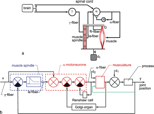
Fig. 8.14 The mammalian system for the control of joint position. (a) simplified illustration of the anatomical situation. (b) The corresponding model circuit. G Golgi organs, R Renshaw cells, xr reference input, d1 and d2 disturbance inputs, y control variable (joint position)
In this feedback system, muscle spindles constitute feedback transducers, comparators, and controllers at the same time. As can be seen from the kind of step response (Fig. 4.11), we have a P-D controller. Its significance could lie in the fact that, in this way, the system can be prevented from becoming unstable, which might otherwise occur due to the mechanical properties of the process (the system is at least of 2nd order since elasticity and inertia are present) and additional delay times due to the limited speed of conduction of the nerves (see Chapter 8.6 ).
Additional sensors exist in this system in the form of the Golgi organs (Fig. 8.14a, G). They are located in the muscle tendons and measure the tension occurring there. We know that, when tension is increased via some interneurons, their effect on the α-motorneurons is inhibitory, but excitatory when the tension is lowered (by antagonistic action). It appears we are dealing with a feedback system designed to keep the tension of the muscles at a constant level. This could be interpreted as a second cascade which compensates disturbance inputs, such as fatigue of the musculature and other properties of the muscles, which affect the direct translation of the spike frequencies of α-fibers into the generation of force. Since, most probably, this influence cannot be described by simple addition, the disturbance input d2 is shown as a second input of the system 'musculature' in Figure 8.14b. The third input in this system takes into account the fact that the force generated by the muscle also depends on its length.
A further cascade of this type is presented by the Renshaw cells (Fig. 8.14a, R) located in the spinal cord, which provide recurrent inhibition to an α-motorneuron. However, we do not want to go into detail concerning this and other elements involved in this feedback system, such as the position receptors in the joints or the tension receptors present in the skin, because little is known so far about the way in which they operate. (One possible explanation of the function of Renshaw cells is found in Adam et al. 1978 ).
The mammalian system to control joint position can be taken as an example that contains several interesting properties of feedback systems. It can be considered as a PD-controller with feedforward of reference input, and is built of several cascades.
Resistance reflexes as described above, where the reflex opposes the movement of a joint, were often discussed in terms excluding the possibility that active movements can be performed because the resistance reflex would immediately counteract such a movement. Thus, it was assumed that resistance reflexes have to be switched off in order to allow for an active movement. However, this is not the only possibility. We have seen that a feedback control system also solves this problem. It provides a resistance reflex when no active movement is intended, i. e., when the reference value is constant, and it performs active movements when the value of the reference input is changed. Another related problem occurs when a sensory input is influenced not only by changes in the outer world, but also by actions of the animal. How can the system decide on the real cause of the changes in the sensory input? One solution to the so-called reafference principle was proposed by v. Holst and Mittelstaedt 1950 (see also Sperry 1950 ). This will be explained using the detection of the direction of a visual object as an example. Figure 8.15a shows a top view of the human eye in a spatially fixed coordinate system. The object is symbolized by the cross. Thus, the absolute position of the cross is given by angle γ. The gaze direction of the eye is given by angle α. The position of the object on the retina, which is the system's only available information, is given by angle β. Angle β changes when the object moves, but also when only the eye is rotated. How can the real angle γ be detected? One possibility is shown in Figure 8.15b. The position α of the eye is controlled by a feedback control system, as shown in the lower part of the figure and represented by the reference input xα and the transfer elements k1 and k2. A second, vision system detects the angle β, the position of the object in a retina-fixed coordinate system. This is shown in the upper part of the figure. The angle β depends on α and γ, due to the geometrical situation according to γ = α + β, or β = γ - α (Fig. 8.15a). This is shown by dashed lines in Figure 8.15 b. How can γ be obtained when the vision system has only β at its disposal? Possible solutions are to use the value α given by the sensory input in the form of k2 α, or to use the efference value k3 xα of the feedback loop. The first case, not shown in Figure 8.15, is simple but can be excluded by experimental evidence. As an alternative, v. Holst and Mittelstaedt proposed to use the copy of the efferent signal xα the "efference copy" instead. According to equation (5) in Chapter 8.3 , we obtain α = k1 /(1 + k1k2) xα. However, in general the vision system does not directly know β but k4β, nor directly xα but k3 xα. Thus, γ can be calculated by γ = k4 β + k3 k1 / (1 + k1k2) xα only if k3 and k4 fulfill particular conditions, a simple case being k 4 = k3 = 1. (For investigation of the dynamics of this and alternative systems, see Varju 1990 ). Thus, with appropriate tuning of the transfer elements k3 and k4, the efference copy, or as it is often called in neurophysiology, the corollary discharge, can solve the problem of distinguishing between sensory signals elicited by the system's own actions and those produced by changes in the environment.
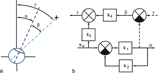
Fig. 8.15 The reafference principle used to visually detect the position of an object, although the eye is movable. (a) The position of the eye within a head-fixed coordinate system is given by α. The position of the object (cross) within an eye-fixed coordinate system is given by β, and within the head-fixed coordinate system by γ. (b) The lower part shows the negative feedback system for the control of eye position (xa reference input, α control variable). The subtraction (γ - α) shown in the right upper part represents the physical properties of the situation. The efference copy signal (passing k3) and the measured value of β are used to calculate γ
A servocontroller can deliberately change the control variable and, at the same time, counteract disturbances. A system working according to the reafference principle, using the efference copy, can distinguish whether a change in sensory input was caused by an motor action of the system itself, or by a change in the environment.
The dynamic behavior of a neuron can be approximated by a relatively simple nonlinear system when the fact that the output of a typical neuron consists of a sequence of action potentials is ignored. If the frequency of these action potentials is not too low, the output value can be regarded as an analog variable. The behavior of such a simplified neuron can be approximated by the differential equation dy/dt = x - f(y), where x is the input excitation and y is the output excitation (= spike frequency) ( Kohonen 1988 ). f(y) is a static nonlinear characteristic the effect of which will be described below. A differential equation can easily be solved numerically by simulating the system on an analog or digital computer, when the equation is transformed into a circuit diagram. How can we find the circuit diagram that corresponds to this differential equation?
Since we have not considered in detail filters having the property of an exact mathematical differentiation, but have treated the much simpler integrators, it is better first to integrate this equation so as to obtain: y = ∫ (x - f(y)) dt. We can now directly plot the corresponding circuit diagram. The characteristic f(y) obtains the output value y. The value f(y) is subtracted from the input x of the system. The resulting difference x - f(y) has to be inserted into an integrator, the output of which provides y. This is shown by the solid arrows in Figure 8.16a. As the output of the integrator and the input of the nonlinear characteristic f(y) comprise the same value, the circuit can be closed (dashed line in Figure 8.16a). Thus, we obtain a system which formally corresponds to a feedback controller. The system might also be considered as a nonlinear "leaky integrator," with f(y) describing the loss of excitation in the system. f(y) should be chosen such that the loss increases overproportionately with the excitation y of the system. This has the effect that the output cannot exceed a definite value. Thus, the system has an implicit saturation characteristic. To make the simulation of a neuron more realistic, one should further introduce a rectifier behind the integrator (not shown in Figure 8.16a) because negative excitation is not possible. Figure 8.16b shows different step responses of this system. In this case, the time constant is the smaller, the greater the output amplitude. Figure 8.16c shows that the sine response of such a system can be asymmetric, as was already found in earlier examples.
As mentioned above, this simulation will produce a sensible replication of the behavior of a neuron only if input excitations above a given value are considered. To make the model also applicable to smaller input values, it could be improved by the introduction of a threshold characteristic at the input.
This model could be used as a simple description of the dynamic properties of a nonspiking neuron, but only as a very rough approximation to the properties of a spiking neuron. In a spiking neuron, information transfer is not continuous. Therefore, a circuit consisting of several spiking neurons can show a behavior which may be unexpected at first sight ( Koch et al. 1989 ). For the investigation of the properties of such circuits, the simulation of a spiking neuron is of interest. Using the simulation procedure given in Appendix II , this can be done simply if it is sufficient to describe the spike by an impulse function of duration of 1 time unit (corresponding to about 1 ms in real time). Figure 8.17 shows the diagram simulating a simple version of a spiking neuron. The first low-pass filter describes the time constant of a dendrite. The Heaviside function represents the threshold which has to be exceeded to produce a spike, and the low-pass filter in the feedback loop represents the refractory effect of a spike being elicited. Figure 8.17b shows an example of how this system reacts to different step-like input functions. As the system contains an implicit nonlinear property, an additional nonlinear characteristic at the input might be necessary to receive the behaviour of a specific neuron.
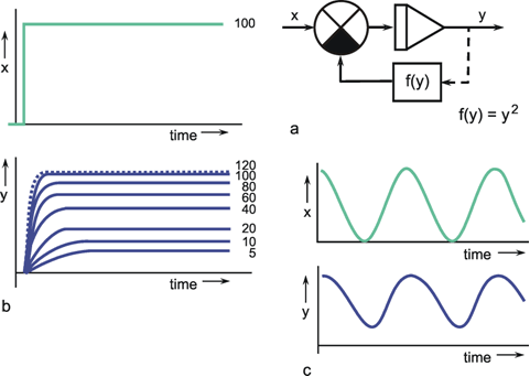
Fig. 8.16 The approximation of the dynamic properties of a neuron. (a) The circuit diagram representing the equation y = ∫ (x - f(y)) dt. (b) Step responses of this system for input steps of different amplitudes. Only one input function (amplitude 100 units) is shown. The responses are marked by the amplitudes of their input functions. The system shows a saturation-like nonlinear behavior. (c) The response to a sine wave. Upper trace: input, lower trace: output. Note that the output function is asymmetrical with respect to a vertical axis
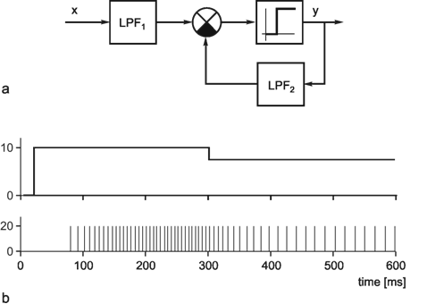
Fig. 8.17 A simple system for the simulation of a spiking neuron. (a) LPF1, and LPF2 represent two low-pass filters. As soon as the threshold of the Heaviside function is overcome, a spike is elicited. (b) Response of such a system to two step-like input functions (first step: from 0 to 10, second step: from 10 to 7.5). Heaviside function: 0 if input < 7, 20 else. Time constants: τ1 = 50 ms, τ2 = 10 ms
As an exercise for solving differential equations as explained above, the reader may like to try to solve the linear differential equations describing a 1st order low-pass filter [dy/dt = (x - y)/τ or y = 1 /τ ∫ (x - y) dt] or a 1st order high-pass filter [d(y-x)/dt = - y/τ or y = x - 1/τ ∫ y dt].
Linear and nonlinear differential equations can be solved by treating them as feedback systems. Two examples are shown which approximate the dynamic properties of nonspiking and of spiking neurons.
As was shown in Chapter 8.3 , difficulties may arise in the calculation of dynamic transfer properties, especially with feedback systems, since the convolution integrals cannot readily be solved. To overcome this problem, we use the Laplace transformation. This is a mathematical formula enabling a transformation of a time function f(t) into a function F(s):
There are a number of simplifications for arithmetic operations with Laplace transformed functions F(s). Addition (and subtraction) are not affected by the transformation. But the latter offers the advantage that the convolution integral y(t) = 0∫tg(t – t’) x(t’)dt' becomes simplified into the product Y(s) = G(s) X(s). Y(s) and X(s) represent the Laplace transformations of y(t) and x(t), and G(s) that of g(t). G(s), the Laplace transformation of the weighting function g(t), is known as the transfer function. Transformations in both directions are achieved by means of tables. The most important transformations are given in the table below.
The following examples serve to illustrate how to use this table. We will start with the example of a simple feedback system (Fig. 8.3), whose filters F1 and F2 are described by the weighting functions g1(t) and g2(t). Since, after the Laplace transformation, only products occur instead of integrals, the equation system (1'), (2'), (3'), (4') described in Chapter 8.3 .
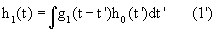


is transformed to
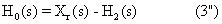

Accordingly, the solution is the following equation:
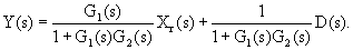
Thus, the transfer function of the closed loop (input: reference input xr, output: controlled variable y) is as follows:
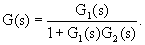
This transfer function is formally obtained very easily by replacing the constants ki in the formulas of Chapter 8.3 by the transfer functions Gi of the corresponding filters. When there is a series connection of several filters, the transfer function of the total system is obtained from the product of the transfer functions of individual filters. When making a parallel connection of two filters and adding their outputs, the transfer function of the total system is obtained by addition of individual transfer functions.
How do we obtain the corresponding weighting function from the transfer function of the closed loop? This will be demonstrated for a selected case (filter F1 is a 1st order low-pass filter with the static amplification factor k1 and the time constant τ, filter F2 is a constant k2). The weighting function of the low-pass filter is g1(t) = k1 e-t/τ. The weighting function of a proportional term without delay, with the amplification factor k2 is as follows: g2(t) = k2. According to the table, we obtain the two transfer functions G1(s) and G2(s) as G1(s) = k1/(τ s + 1) and G2(s) = k2. For the transfer function of the closed loop G(s), we then have
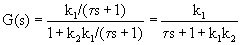
This has to be reformulated in such a way that it takes a form which can be found in the table of the Laplace functions. This can be done as follows:
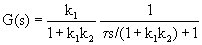
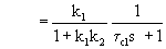
with
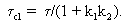
The corresponding weighting function can now be obtained by a transformation in the reserve direction by means of the table. A comparison of this transfer function with those given in the table immediately shows that this is the transfer function of a 1 st order low-pass filter with the time constant τcl, and the static amplification factor k1/(1 + k1, k2).
In the second example a system with positive feedback, a proportional element G1(s) = k1 and a high-pass filter in the feedback loop with G2(s) = k2 τs/(τs + 1) can be calculated as follows
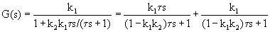
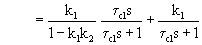
with
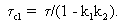
This shows that the system has the same properties as an parallel connection of a high-pass filter (first term) having a dynamic amplification factor of k1 /(1 – k1 k2) (i. e. k1 k2 has to be smaller than 1) and a low-pass filter (second term). Both filters have the same time constant τcl. The output of these filters is added as shown in Figure 4.8a.
A detailed discussion of the preconditions to be fulfilled by a function to enable a Laplace transformation is not intended within the present framework. We are stating, though, that the transformation is permissible for all functions listed in the table. If, as in the first part of the table, general references to functions are made, such as y(t) or Y(s), all functions contained in the table may be used. See Abramowitz and Stegun (1965) , for example, for more detailed tables, and DiStefano et al. (1967) for a detailed description of Laplace transformation.


Weighting functions:


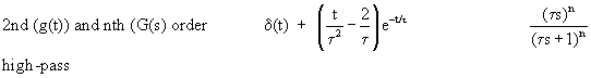
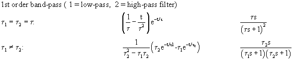

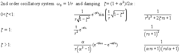
Linear and nonlinear systems can be simulated in simple ways by means of digital programs. As a frame such a program requires a loop, with the loop variable t representing the time. By each iteration the time increases by one unit. Within the loop it is simple to simulate an integrator. This is done by the line xout = xout + xin. As low-pass filters and high-pass filters can be constructed by feedback systems with integrators ( Chapter 8.5 ), their simulation requires two or three program lines as shown in the example below. The output values can be subject to arbitrary continuous or non-continuous nonlinear characteristics.
By combining the output values in appropriate ways, arbitrary parallel and serial connections can be simulated. The following small C-program shows as an example the parallel connection of a low-pass and a high-pass filter. The summed output passes a rectifier, then a 2nd order oscillatory low-pass filter and finally a pure time delay. As input in this case a step function is chosen. Variables beginning with a y represent the output values of the system, variables starting with an aux represent the auxiliary variables. tau, omega, zeta represent time constant, eigenfrequency, and damping factor ζ of the filters, respectively, as described in Chapters 4.1 , 4.3 , and 4.9 . The dead time is given by T.
main {
for (t = 1; t < 500; t++) {
/* input step function */
if (t < 20) input = 0; else input = 10.;
/* low-pass filter*/
aux_lpf = aux_lpf + input - y_lpf;
y_lpf = aux_lpf/tau_lpf;
/* high-pass filter*/
aux_hpf = aux_hpf + y_hpf;
y_hpf = input - aux_hpf/tau_hpf;
/* summation */
sum = y_hpf + y_lpf;
/* rectifier */
if (sum < 0.) sum = 0.;
/* 2nd order oscillatory low-pass filter */
input = sum;
aux0_osc = input1 + omega*aux3 osc + zeta* aux2_osc;
aux1_osc = aux1_osc + aux0_osc;
aux2_osc = - aux1_osc;
aux3_osc = aux3_osc + aux2_osc;
aux4_osc=- aux3_osc;
y_osc = aux4_osc;
/* pure time delay*/
input2 = y_osc;
y_ptd = buffer[T];
if (T > 0)
{for (i = T; i > 0; i--) buffer[i] = buffer [i - 1];}
buffer[0] = input2;
/* output */
output = y_ptd;}/* end of loop */
} /* end of main */
Concepts are understood best, if the underlying ideas are not only verbally explained, but if, in addition, comprehension is supported by practical exercises. Whereas for the second part of the book, which deals with different types of neural networks, specifically designed software is provided, for the first part, i.e. Chapters 1 – 8, a general solution, the software package tkCybernetics is recommended. tkCybernetics, developed by Th. Roggendorf, allows on a graphical interface to easily and quickly construct different systems containing linear filters and nonlinear characteristics and the selection of different input functions.
The following exercises are designed to be performed with the simulation tool tkCybernetics .
A general advice before you start: Having a comfortable software package for the simulation of systems bears the following danger. One is inclined to first construct the system, then run it, look at the system’s response, and only then try to understand what has happened. A much better way is to first construct the system, but before starting the input function, try to predict the probable result, for example by plotting a rough sketch of the expected response. Only after you have done this, start the input function and compare the result with your prediction. This is not as easy as the first approach, but helps dramatically to improve your understanding of the properties of dynamic systems. So, in parallel to your computer, always use paper and pencil when you are doing simulation exercises.
1) Investigate step response, ramp response, pulse response and frequency response (Bode plot) of:
a. Low pass filter (e.g. time constant = 30 units) (see Chapter 4.1 )
b. High pass filter (see Chapter 4.2 ).
c. 2nd order low-pass filter (see Chapter 4.3 ).
d. 2nd order high-pass filter (see Chapter 4.4 ).
e. Integrator (see Chapter 4.8 ).
f. Serial combination of low-pass and high-pass filter (see Chapter 4.5 ). Try different time constants for both filters.
g. Parallel combination of low-pass and high-pass filter (see Chapter 4.6 ). Try different time constant for both filters and vary the gain in the branch of the high-pass filter, for instance.
2) Investigate the step responses of the circuits shown in Fig. 4.8 .
3) Systems with feedback connections:
a. Investigate the step responses of a circuit as shown in Fig. 8.2 , but without a disturbance input. Vary the values of the constants k1 and k2 between 0 and 5.
b. Replace one constant by a filter, e.g. a low-pass filter. Vary the values of the constants k1 and k2.
4) Repeat exercise 3) by applying a positive feedback connection instead of a negative one!
5) Negative feedback controller:
Test the six examples given in Fig. 8.8 by varying the values of the constants (note that some of these tasks have already been solved in the former exercises.) In particular challenge the stability of the system, by varying the constants (gain factors) and adding further low-pass filters of an order being high enough.
6) Nonlinear properties:
a. Apply a sine function to a concave or convex nonlinear characteristic (see Chapter 5 ).
b. Investigate the different serial connection of a linear filter and a nonlinear characteristic as shown in Figs. 6.2 and 6.3 . Test step response and the response to a sinusoidal input.
c. Try a simulation of the system illustrated in Fig. 6.4 .
7) Feedback systems with nonlinear properties.
a. Simulate the system illustrated in Fig. 8.16 .
b. Simulate the system illustrated in Fig. 8.17 .
Abramowitz, M., Stegun, I. (1965): Handbook of Mathematical Functions. Dover Publications, New York
Adam, D., Windhorst, U., Inbar, G.F. (1978): The effects of recurrent inhibition on the cross-correlated firing pattern of motoneurons (and their relation to signal transmission in the spinal cord-muscle channel). Biol. Cybernetics 29, 229-235
Amari, S. (1967): Theory of adaptive pattern classifiers. IEEE Trans., EC-16, No. 3, 299-307
Amari, S. (1968): Geometrical theory of information (in Japanese). Kyoritsu-Shuppan, Tokyo
Amari, S. (1977): Dynamics of pattern formation in lateral-inhibition type neural fields. Biol. Cybern. 27, 77-87
Amari, S., Arbib, M.A. (1982): Competition and Cooperation in Neural Nets. Springer Lecture Notes in Biomathematics Nr 45
Arbib, M.A. (1995): Schema theory. In: M.A. Arbib (ed.) The Handbook of Brain Theory and Neural Networks. MIT Press, Bradford Book, Cambridge, Mass, 1995
Baldi, P., Heiligenberg, J.M. (1988): How sensory maps could enhance resolution through ordered arrangements of broadly tuned receivers. Biol. Cybern. 59,313-318
Barto, A.G., Sutton, R.S., Brouwer, P.S. (1981): Associative search network: a reinforcement learning associative memory. Biol. Cybern. 40, 201 -211
Barto, A.G., Sutton, A.G., Watkins, C. (1990): Sequential decision problems and neural networks. In: M. Gabriel, J.W. Moore (eds.) Advances in neural information processing systems. Morgan Kaufmann 1990, 686-693
Bässler, U. (1983): Neural basis of elementary behavior in stick insects. Springer, Berlin, Heidelberg, New York
Bässler, U. (1993): The femur-tibia control system of stick insects - a model system for the study of the neural basis of joint control. Brain Res. Rev. 18, 207-226
Bechtel, W., Abrahamsen, A.A. (1990): Connectionism and the mind: an introduction to parallel processing in networks. Basil Blackwell, Oxford
Beckers, R., Deneubourg, J.L, Goss, S. (1992): Trails and U-turns in the selection of a path by the ant Lasius niger. J. of Theor. Biol. 159, 397-415
Bernstein, N. (1967): The co-ordination and regulation of movements. Pergamon Press Ltd.
Brooks, R.A. (1986): A robust layered control system for a mobile robot. J. Robotics and Automation 2, 14-23
Brooks, R.A. (1989): A robot that walks: emergent behaviours from a carefully evolved network. Neural Computation I, 253-262
Cabanac, M. (1992): Pleasure: the common currency. J. Theor. Biol. 155, 173-200
Camazine, S., Deneubourg, J.-L., Franks, N. R., Sneyd, J., Theraulaz, G., Bonabeau, E. (2003) Self-organization in biological systems. Princeton Univ. Press, Princeton
Carpenter, G.A., Grossberg, S. (1987): A massively parallel architecture for a self-organizing neural pattern recognition machine. Computer Vision, Graphics, and Image Processing 37, 54-115
Chapman, K.M.. Smith, R.S. (1963): A linear transfer function underlying impulse frequency modulation in a cockroach mechanoreceptor. Nature 197, 699-700
Clynes, M. (1968): Biocybernetic principles and dynamic asymmetry: unidirectional rate sensitivity. In: H. Drischel (ed.) Biokybernetik. Vol. 1, Fischer, Jena 29-49
Cruse, H. (1979): Modellvorstellungen zu Bewußtseinsvorgängen. Naturw. Rdschau 32, 45-54
Cruse, H. (1981): Biologische Kybernetik. Verlag Chemie. Weinheim, Deerfield Beach, Basel
Cruse, H. (1990): What mechanisms coordinate leg movement in walking arthropods? Trends in Neurosciences 13, 1990, 15-21
Cruse, H. (2003): The evolution of cognition – a hypothesis. Cog. Science 27, 135-155
Cruse, H. (2002). Landmark-based navigation. Biol. Cybernetics 88, 425-437
Cruse, H., Bartling, Ch., Kindermann, Th. (1995): Highpass filtered positive feedback: decentralized control of cooperation. In: F. Moran, A. Moreno, J.J. Merelo, P. Chacon (eds.) Advances in Artificial Life. Springer, 668-678
Cruse, H., Dean, J., Heuer, H., Schmidt, R.A. (1990): Utilisation of sensory information for motor control. In: 0. Neumann, W. Prinz (eds.) Relationships between perception and action. Springer, Berlin, 43-79
Cruse, H., Dean, J., Ritter, H. (1995): Prärationale Intelligenz. Spektrum d. Wiss. 111-115
Cruse, H., Müller-Wilm, U., Dean, J. (1993): Artificial neural nets for controlling a 6-legged walking system. In: J.A. Meyer, H. Roitblat, S.Wilson (eds.) From animals to animats 2. 52-60. MIT Press, Cambridge MA
Cruse, H., Steinkühler, U. (1993): Solution of the direct and inverse kinematic problem by a unique algorithm using the mean of multiple computation method. Biol. Cybern. 69, 345-351
Daugman, J.G. (1980): Two-dimensional spectral analysis of cortical receptive field profiles. Vision Res. 20, 847, 856
Daugman, J.H. (1988): Complete discrete 2-D Gabor transforms by neural networks for image analysis and compression. IEEE Transact. on acoustics, speech, and signal processing. 36, 1169-119
Dean, J. (1990): Coding proprioceptive information to control movement to a target: simulation with a simple neural network. Biol. Cybern. 63, 115-120
Dean, J., Cruse, H., and Ritter, H. (2000): Prerational Intelligence: Interdisciplinary perspectives on the behavior of natural and artificial systems. Kluwer Press, Dordrecht
Deneubourg, J.L, Goss, S. (1989): Collective patterns and decision making. Ethology, Ecology and Evolution 1, 295-311
Dijkstra, S., Denier van der Gon, J.J. (1973): An analog computer study of fast isolated movements. Kybernetik 12,102 -110
DiStefano, 111, Joseph J., Stubberud, Allen R., Williams, Ivan J. (1967): Theory and Problems of Feedback and Control Systems with Applications to the Engineering, Physical, and Life Sciences. McGraw Hill, New York, St. Louis, San Francisco, Toronto, Sydney
Eckhorn, R., Bauer, R., Jordan, W., Brosch, M., Kruse, W., Munk, M., Reitboeck, H.J. (1988): Coherent oscillations: a mechanism of feature linking in the visual cortex? Multiple electrode and correlation analysis in the cat. Biol. Cybernetics 60, 121 - 130
Eibl-Eibesfeldt, I. (1980): Jumping on the sociobiology bandwagon. The Behavioral and Brain Sciences 3, 631-636
Elman, J.L. (1990): Finding structure in time. Cognitive Science 14, 179-211
Engel, A.K., König, P., Kreiter. A.K., Schillen, TB., Singer, W. (1992): Temporal coding in the visual cortex: new vistas on integration in the nervous system. Trends in Neurosciences 15, 218-226
Exner, S. (1894): Entwurf einer physiologischen Erklärung der psychischen Erscheinungen. 1. Ted. Deuticke, Leipzig, 37-140
Fahlman, S.E., Lebiere, C. (1990): The cascade correlation learning architecture. In: D.S. Touretzky (ed.) Advances in neural information processing systems 2. Morgan Kaufman Pub. San Mateo, CA, 524-532
Fenner, F.J., Gibbs, E.P.J., Murphy, EA., Rott, R., Studdert, M.J., White, D.O. (1993): Veterinary Virology. Academic Press. San Diego, New York, Boston
Franceschini, N., Riehle, A., Le Nestour, A. (1989): Directionally selective motion detection by insect neurons. In: Stavenga, Hardie (eds.) Facets of Vision. Springer, Berlin, Heidelberg, 360-390
Fukushima, K. (1975): Cognitron: a self-organizing multilayered neural network. Biol. Cybern. 20, 121-136
Fukushima, K. (1980): Neocognitron: a self-organizing neural network model for a mechanism of pattern recognition unaffected by shift in position. Biol. Cybern. 36,193-202
Haken, H. (ed.) (1973): Synergetik. Teubner, Stuttgart
Hartmann, G., Wehner, R. (1995): The ant's path integration system: a neural architecture. Biol. Cybern. 73, 483-497
Hassenstein, B. (1958 a): Über die Wahrnehmung der Bewegung von Figuren und unregelmäßigen Helligkeitsmustern am Rüsselkäfer Chlorophanus viridis. Zeitschrift für vergleichende Physiologie 40, 556-592
Hassenstein, B.(1958 b): Die Stärke von optokinetischen Reaktionen auf verschiedene Mustergeschwindigkeiten (bei Chlorophanus viridis). Z. Naturforschg. 12 b, 1-6
Hassenstein, B. (1959): Optokinetische Wirksamkeit bewegter periodischer Muster (nach Messungen am Rüsselkäfer Chlorophanus viridis). Z. Naturforschg. 14b, 659-674
Hassenstein, B. (1966): Kybernetik und biologische Forschung. Handbuch der Biologie, vol. 1/2, pp. 629-719. Akademische Verlagsgesellschaft Athenaion. Frankfurt/M.
Hassenstein, B. (1971): Information and control in the living organism. Chapman and Hall, London
Hassenstein, B., Reichardt, W. (1953): Der Schluß von den Reiz-Reaktions-Funktionen auf System-Strukturen. Z. Naturforsch. 86, 518-524
Hassenstein, B., Reichardt, W. (1956): Systemtheoretische Analyse der Zeit-, Reihenfolgen- und Vorzeichenauswertung bei der Bewegungsperzeption des Rüsselkäfers Chlorophanus. Z. Naturforschg. 11 b, 513-524
Hebb, D.O. (1949): The organization of behavior. Wiley, New York
Heisenberg, M., Wolf, R(1988): Reafferent control of optomotor yaw torque in Drosophilia melanogaster. J. Comp. Physiol. 163:373-388
Hertz, J., Krogh, A., Palmer, R.G. (1991): Introduction to the theory of neural computation. Addison-Wesley Pub., Redwood City
Hinton, G.E., McClelland, J.L., Rumelhart, D.E. (1986): Distributed representation. In: D.E. Rumelhart, J.L. McClelland (eds.) Parallel Distributed Processing, Vol. 1, MIT Press, Cambridge MA, 77-109
Holland, J.H. (1975): Adaptation in natural and artificial systems. Univ. of Michigan Press (2nd edition MIT Press, 1992)
Holst, E.v. (1950a): Die Arbeitsweise des Statolithenapparates bei Fischen. Zeitschr. Vergl. Physiol. 32, 60-120
Holst, E.v. (1950b): Die Tätigkeit des Statolithenapparats im Wirbeltierlabyrinth. Naturwissenschaften 37, 265-272
Holst, E.v. (1957): Aktive Leistungen der menschlichen Gesichtswahrnehmung. Studium Generale 10, 231-243
Holst, E.v., Mittelstaedt, H. (1950): Das Reafferenzprinzip: Wechselwirkungen zwischen Zentralnervensystem und Peripherie. Naturwissenschaften 37, 464-476
Hopfield, J.J. (1982): Neural networks and physical systems with emergent collective computational abilities. Proc. Natl. Acad. Sci. 79, 2554-2558
Hopfield, J.J. (1984): Neurons with graded response have collective computational properties like those of two-state neurons. Proc. Natl. Acad. Sci. 81, 3088-3092
Hopfield, J.J., Tank, D.W. (1985): "Neural" computation of decisions in optimization problems. Biol. Cybern. 52, 141-152
Iles, J.F., Pearson, K.G. (1971 ): Coxal depressor muscles of the cockroach and the role of peripheral inhibition. J. Exp. Biol. 55,151 -164
Jacobs, R.A., Jordan, M.1., Nowlan, S.J., Hinton, G.E. (1991): Adaptive mixtures of local experts. Neural Computation 3, 79-87
Jaeger, H., Haas, H. (2004): Harnessing Nonlinearity: Predicting Chaotic Systems and Saving Energy in Wireless Communication. Science, April 2, 2004, 78-80. [Preprint including supplementary material: http://www.faculty.iu-bremen.de/hjaeger/pubs/ESNScience04.pdf ]
Jordan, M.L (1986): Attractor dynamics and parallelism in a connectionist sequential machine. In: Proceedings of the eighth annual conference of the cognitive science society. (Amherst 1986) Hillsdale, Earlbaum, 531 - 546
Jordan, M.L (1990): Motor learning and the degrees of freedom problem. In: M. Jeannerod (ed.) Attention and Performance XIII. Hillsdale, NJ, Earlbaum, 796-836
Jordan, M.L, Jacobs, R.A. (1992): Hierarchies of adaptive experts. In: J. Moody, S. Hanson, & R. Lippmann, (eds.) Neural Information Systems, 4. Morgan Kaufmann, San Mateo, CA
Jones, W.P., Hoskins, J. (1987): Backpropagation: a generalized delta learning rule. Byte 155-162
Kandel, E.R.. Schwartz, J.H., Jessel, T.M. (2000): Principles of neural science. Elsevier, New York, Amsterdam, Oxford
Kawato, M., Gomi, H. (1992): The cerebellum and VOR/ OKR learning model. Trends in Neurosciences 15,455 - 453
Kindermann, Th., Cruse, H., Dautenhahn, K. (1996): A fast, three layered neural network for path finding. Network: Computation in Neural Systems 7, 423-436
Koch, U.T., Bässler, U., Brunner, M. (1989): Non-spiking neurons suppress fluctuations in small networks. Biol. Cybern. 62, 75-81
Kohonen, T. (1982): Self-organized formation of topologically correct feature maps. Biol. Cybern. 43, 59-69
Kohonen, T. (1988): An introduction to neural computing. Neural Networks 1, 3-16
Kohonen, T. (1989): Self-organization and associative memory. Springer Series in Information Sciences. Springer Verlag, 3rd edition
Koza. J.R. (1992): Genetic programming: A paradigm for genetically breeding computer population of computer programs to solve problems. MIT Press, Cambridge MA
Kühn, S., Beyn, W.-J., Cruse, H. (2007) Modeling memory function with recurrent neural networks consisting of Input Compensation units. I. Static Situations. Biol. Cybernetics 96, 455- 470
Kühn, S., Cruse, H. (2007) Modelling memory function with recurrent neural networks consisting of Input Compensation units. II. Dynamic Situations. Biol. Cybernetics 96, 471- 486
Le Cun, Y. (1985): Line procedure d'apprendissage pour reseau a seuil assymetrique. In: Cognitiva 85: A la frontiere de I'intelligence artificielle des sciences de la connaissance des neurosciences. Paris 1985, 599604. Paris CESTA
Levin, E. (1990): A recurrent network: limitations and training. Neural Networks 3, 641-650
Linder, C. (2005) Self-organization in a simple task of motor control based on spatial encoding. Adaptive Behavior 13, 189-209
Littmann, E., Ritter, H. (1993): Generalization abilities of cascade network architectures. In C.L. Giles, S.J. Hanson, J.D. Cowan (eds.) Advances in neural information processing systems 5. Morgan Kaufman Pub., San Mateo, CA, 188-195
Lorenz, K. (1950): The comparative method in studying innate behavior patterns. Symp. Soc. Exp. Biol. 221 - 268
Maass, W., Natschläger, T. and Markram. H. (2002): Real-time computing without stable states: A new framework for neural computation based on perturbations. Neural Computation, 14(11):2531-2560 http://www.lsm.tugraz.at/papers/lsm-nc-130.pdf
Maes, P. (1991): A bottom-up mechanism for behavior selection in an artificial creature. In: J.A. Meyer, S.W. Wilson (eds.) From animals to animats. Bradford Book, MIT Press, Cambridge Mass, London, 238-246
Makarov, V.A., Song, Y., Velarde, M.G., Hübner, D., Cruse, H. (2008): Elements for a general memory structure: Properties of recurrent neural networks used to form situation models. Biol. Cybern. 98, 371-395
von der Malsburg, Ch. (1973): Self-organization of oriented sensitive cells in the striate cortex. Kybernetik 14, 85-100
von der Malsburg, Ch. (1981): The correlation theory of brain function, Internal report 81-2, Göttingen, Germany: Max Planck Institut fur Biophysikalische Chemie. Reprinted in: Models of Neural Networks (K. Schulten, H.J. van Hemmen, eds.) Springer, 1994
von der Malsburg, Ch., Buhmann, J. (1992): Sensory segmentation with coupled neural oscillators. Biol. Cybern. 67, 233-242
Marmarelis, P.Z., Marmarelis, V.Z. (1978): Analysis of physiological systems: the white noise approach. Plenum Press, New York
Martinetz, T., Ritter, H., Schulten, K. (1990): Three-dimensional Neural Net for Learning Visuomotor-Coordination of a Robot Arm. IEEE-Transact. on Neural Networks 1,131-136
McFarland. D., Bösser, Th. (1993): Intelligent behavior in animals and robots. Bradford Book, MIT Press, Cambridge MA
Meinhardt, H. (1995): The algorithmic beauty of sea shells. Springer, Heidelberg
Milhorn, H.T. (1966): The application of control theory to physiological systems. Saunders, Philadelphia
Milsum, IT. (1966): Biological control systems analysis. McGraw Hill, New York
Minsky, M. (1985): The society of mind. Simon and Schuster, New York
Minsky, M.L., Papert, S.A. (1969): Perceptrons. MIT Press, Cambridge
Möhl, B. (1989): "Biological noise" and plasticity of sensorimotor pathways in the locust flight system. J. comp. Physiol. A 166, 75 -82
Möhl, B. (1993): The role on proprioception for motor learning in locust flight. J. Comp. Physiol. A 172, 325-332
http://dx.doi.org/10.1007/11840817_63 Mohan, V., Morasso, P. (2006): A Forward / Inverse Motor Controller for Cognitive Robotics. ICANN (1) 2006, 602-611
Nauck D, Klawonn F, Borgelt C, Kruse R (2003) Neuronale Netze und Fuzzy Systeme. Braunschweig/ Wiesbaden: Vieweg-Verlag.
Oppelt, W. (1972): Kleines Handbuch technischer Regelvorgange. Verlag Chemie, Weinheim
Pfeifer, R. (1995): Cognition - perspectives from autonomous agents. Robotics and Autonomous Systems 15, 47-69
Pfeifer, R., and Verschure, P.F.M.J. (1992): Distributed adaptive control: a paradigm for designing autonomous agents. In: Towards a practice of autonomous systems: Proc. of the First European Conference on Artificial Life. MIT Press, Cambridge, Mass. 21-30
Pichler, J., Strauss, R. (1993): Altered spatio-temporal orientation in ellipsoid-body-open, a structural central complex mutant of Drosophila melanogaster. In: Elsner, N., Heisenberg, M. (eds.) Gene, Brain, Behavior. Proceedings of the 21st Göttingen Neurobiology Conference. p. 813. Stuttgart, Thieme
Ratliff, E (1965): Mach Bands: Quantitative Studies on Neural Networks in the Retina. Holden-Day, San Francisco, London, Amsterdam
Rechenberg, L (1973): Evolutionsstrategie: Optimierung technischer Systeme nach Prinzipien der biologischen Evolution. Fromman-Holzboog. Stuttgart
Reichardt, W. (1957): Autokorrelationsauswertung als Funktionsprinzip des Zentralnervensystems. Z. Naturforsch. 12 b, 448 -457
Reichardt, W. (1973): Musterinduzierte Flugorientierung der Fliege Musca domestica. Naturwissenschaften 60, 122-138
Reichardt, W., MacGinitie, G. (1962): Zur Theorie der lateralen Inhibition. Kybernetik 1, 155-165
Riedmiller, M., Braun, H. (1993): A direct adaptive method for faster backpropagation learning: the RPROP Algorithm. Proceedings of the IEEE Int. Conf. on Neural Networks (IBNN), 586-591
Ritter, H., Kohonen, T. (1989): Self-Organizing Semantic Maps. Biol. Cybern. 61, 241-254
Ritter, H., Martinez, T., Schulten, K. (1989): Topology conserving maps for learning visuomotor coordination. Neural Networks 2, 159-168
Ritter, H., Martinetz, Th., Schulten, K. (1992): Neural Computation and Self-organizing Maps. Addison Wesley, 1 st revised english edition
Rizzolatti, G. (2005): The mirror neuron system and its function in humans. Anat. Embryol. 210(5–6) 419–421
Rosenblatt, E (1958): The perceptron: a probabilistic model for information storage and organization in the brain. Psychol. Rev. 65, 386-408
Rumelhart, D.E., Hinton, G.E., Williams, R.J. (1986): Learning internal representations by back-propagating errors. Nature 323, 533-536
Rumelhart, D.E., McClelland, J.L. (1986): Parallel Distributed Processing, Vol. 1, Bradford Book, MIT Press, Cambridge Mass, London
Schilling, M., Cruse, H. (2008): The evolution of cognition – from first order to second order embodiment. In: Modeling Communication with robots and virtual humans. I. Wachsmuth, G. Knoblich (eds.) Springer, Berlin, Lecture Notes in Artificial Intelligence, pp. 77-108
Schmidt, R. E. (1972): Grundriß der Neurophysiologie. Springer, Berlin, Heidelberg, New York
Schmidt, R. E. (1973): Grundriß der Sinnesphysiologie. Springer, Berlin, Heidelberg, New York
Schöner, G. (1991): Dynamic theory of action-perception patterns: the "moving room" paradigm. Biol. Cybern. 64, 455-462
Sejnowski, T. J., Tesauro, G. (1989): The Hebb rule for synaptic plasticity: algorithms and implementations. In: Byrne, J.H., Berry, W.O. (eds.) Neural models of plasticity: Experimental and theoretical approaches., Academic Press, pp. 94-103
Shiffrar, M. (2001): Movement and event perception. In: Goldstein, B. (ed.), The Blackwell Handbook of Perception. Blackwell Publishers, Oxford. pp. 237–272
Spekreijse, H., Oosting, H. (1970): Linearizing: a method for analysing and synthesizing nonlinear systems. Kybernetik 7, 22-31
Sperry, R. W. (1950): Neural basis of the spontaneous optokinetic response produced by visual inversion. J. Comp. Psychol. 43, 482-499
Steels, L. (1994a): Emergent functionality in robotic agents through on-line evolution. In: R. Brooks, P. Maes (eds.) Proceedings of the IV. MIT Press, Cambridge MA
Steels, L. (1994b): The artificial life roots of artificial intelligence. Artificial Life 1, 75-110
Steil, J.J. (1999) Input-Output Stability of Recurrent Neural Networks. Göttingen: Cuvillier Verlag.
Stein, R.B. (1974): Peripheral control of movement. Physiol. Rev. 54, 215-243
Steinbuch, K. (1961): Die Lernmatrix. Kybernetik 1, 36-45
Steinkühler, U., Cruse, H. (1998): A holistic model for an internal representation to control the movement of a manipulator with redundant degrees of freedom. Biol. Cybernetics 79, 457-466
Tani, J. (2003): Learning to generate articulated behaviour through the bottom-up and the top-down interaction process. Neural Networks 16, 11-23
Tani J, Nolfi S (1999) Learning to perceive the world articulated: an approach for hierarchical learning in sensory-motor systems. Neural Networks 12: 1131-1141.
Tani, J., Ito, M., Sugita, Y. (2004): Self-organization of distributedly represented multiple behaviour schemata in a mirror system: rebviews of robot experiments using RNNPB. Neural Networks 17, 1273-1289
Tank, D.W., Hopfield, J.J. (1987): Collective computation in neuron-like circuits. Scientific American 257, 104
Thorson, J. (1966): Small signal analysis of a visual reflex in the locust 11. Frequency dependence. Kybernetik 3, 53-66
Varju, D. (1962): Vergleich zweier Modelle für laterale Inhibition. Kybernetik 1, 200-208
Varju, D. (1965): On the theory of lateral Inhibition. Consiglio nazionale delle Ricerche, Rome, 1-26
Varju, D. (1977): Systemtheorie. Springer, Berlin, Heidelberg, New York
Varju, D. (1990): A note on the reafference principle. Biol. Cybern. 63, 315-323
Wagner, R. (1960): Über Regelung von Muskelkraft und Bewegungsgeschwindigkeit bei der Willkürbewegung. Z. Biol. 111, 449-478
Wehner, R. (1987): "Matched filters" - neural models of the external world. J. Comp. Physiol. A 161, 511-531
Werbos, P.J. (1974): Beyond regression: new tools for prediction and analysis in the behavioral sciences. Ph.D. Thesis, Harvard University
Williams, R.J. (1992): Simple statistical gradient-following algorithms for connectionist reinforcement learning. Machine Learning 8, 229-256
Williams, R.J. and D. Zipser (1989): A learning algorithm for continually running fully recurrent neural networks. Neural Computation, 1, 270-280.
Willshaw, D.J., von der Malsburg, C. (1976): How patterned neural connections can be set up by self-organization. Proceedings of the Royal Society of London B 194, 431-445
Wilson, S.W. (1987): Classifier systems and the animat problem. Machine Learning 2,199 -228
Wolpert, D.M., Kawato, M. (1998): Multiple paired forward and inverse models for motor control. Neural Networks 11, 1317-1329
License
Any party may pass on this Work by electronic means and make it available for download under the terms and conditions of the Digital Peer Publishing License. The text of the license may be accessed and retrieved via Internet at http://www.dipp.nrw.de/lizenzen/dppl/dppl/DPPL_v2_en_06-2004.html