[ view printable version ]

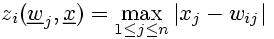
A biological neuron can be technically modeled as a formal, static neuron, which is the elementary building block of many artificial neural networks. Even though the complex structure of biological neurons is extremely simplified in formal neurons, there are principal correspondences between them: An input function x of the formal neuron i corresponds to the incoming activity (e.g. synaptic input) of the biological neuron, the weight w represents the effective magnitude of information transmission between neurons (e.g. determined by synapses), the activation function z_i=f(x,w_i) describes the main computation performed by a biological neuron (e.g. spike-rates or graded potentials) and the output function y_i=f(z_i) corresponds to the overall activity transmitted to the next neuron in the processing stream (see Fig. 1).

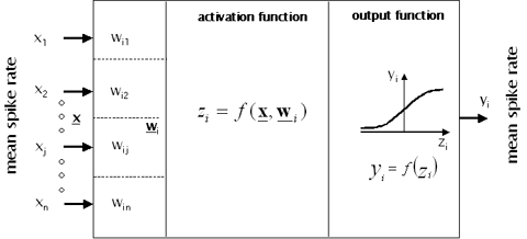
Figure 1: Basic elements of a formal, static neuron.

The activation function z_i=f(x,w_i) and the output function y_i=f(z_i) are summed up with the term transfer functions. Important transfer functions will be described in the following in more detail:

The activation function z_i=f(x,w_i) connects the weights w_i of a neuron i to the input x and determines the activation or the state of the neuron. Activation functions can be divided into two groups, the first based on dot products and the second based on distance measures.

The activation of a static neuron in a network net_i based on the dot product is the weighted sum of inputs:

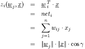(1)

In order to interpret this activation, it has to be considered that an equation of the form

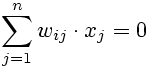(2)

defines a (hyper-) plane through the origin of a coordinate system. The activation z_i=f(x,w_i) is zero, when an input x is located on a hyperplane, which is 'spanned' by the weights w_i and w_n. Activation increases (or, respectively decreases) with increasing distance from the plane. The sign of the activation indicates on which side of the plane the input x is. Thus, the sign separates the input space into two dimensions.

A general application of the hyperplane (in other than the origin position) requires that each neuron i has a threshold Θ_i. As a result, the hyperplane can be described as:

(3)

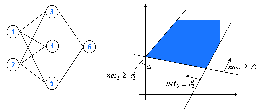
In order to understand the application of hyperplanes in artificial neural networks, consider a net of neurons with n input neurons (net 1 and net 2 in Fig. 2) as well as trainable weights (hidden neurons; net 3, net 4 net 5 in Fig. 2) and one output neuron (net 6 in Fig. 2). Assume a limited interval of inputs [0, 1]. The n-dimensional input space is separated by (n-1)-dimensional hyperplanes that are determined by the hidden neurons. Each hidden neuron defines a hyperplane (a straight line in the 2D case of Fig. 2 right) and separates two classes of inputs. By combining hidden neurons very complex class separators can be defined. The output neuron can be described as another hyperplane inside the space defined by the hidden neurons, which allows a connection between subspaces of the input space (in Fig. 2 right, for example, a network representing the logical connection AND between two inputs is shown: if input 1 AND input 2 are within the colored area, the output neuron is activated).

Activation functions based on dot products should be combined with output functions that account for the sign, because otherwise the discrimination of subspaces separated by hyperplanes is not possible.

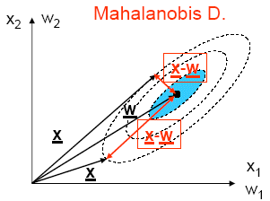
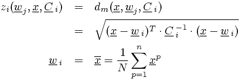
Alternatives to activation functions based on dot products are activation functions based on distance measures. The weight vectors of neurons represent the data in the input space. The activation of a neuron i is computed from the distance of the weight w_i from the input x.Determining this distance is possible by applying different measures. A selection is presented in the following:

The activation of a neuron is determined exclusively by the weight vectors' spatial distance from the input. The direction of the difference vector x-w_i is insignificant. Two cases are considered here: the Euclidian Distance that is applied in cases of symmetrical input spaces (data with 'spherical' distributions that are equally distributed in all directions) and the more general Mahalanobis Distance that also accounts for cases of asymmetric input spaces with the covariance matrix C_i. (In the simulation, the matrix can be influenced by σ₁, σ₂ and φ.)

(4)

The activation of neurons is determined by the maximum absolute value (modulus) of the components of the difference vector x-w_i.

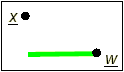
(5)

The activation of neurons corresponds to the minimal absolute value of the components of the difference vector x-w_i.

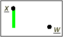
(6)

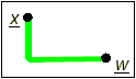
The Manhattan distance results from the activation of neurons determined by the sum of the absolute values of the vector components x-w_i.

(7)

The output functions define the output y_i of a neuron depending on the activation z_i(x,w_i). In general, monotonically increasing functions are applied. These functions bring about an increasing activity for an increasing input as it is often assumed for biological neurons in the form of an increasing spike-rate (or graded potential) for increasing synaptic input. By defining an upper threshold in the output functions, the refractory period of biological neurons can be considered in a simple form. A selection of output functions will be presented in the following:

(8)

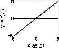
The identity function does not apply thresholds and results in a an output y_i that is identical to the input z_i(x,w_i).

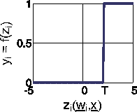
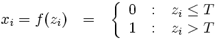
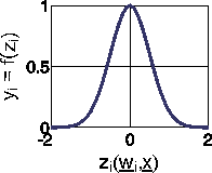
The Heaviside function (as temporal function known as 'step function') is used to model the classic 'All-or-none' behaviour. It resembles a ramp function (see below), but changes the function value abruptly when a threshold value T is reached.

(9)

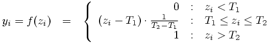
The ramp function combines the heaviside function with a linear output function. As long as the activation is smaller than the threshold value T₁, the neuron shows the output y_i=0; if the activation exceeds the threshold value T₂ The output is y_i=1. The neuron's output for activations in the interval between the two threshold values T₁<z_i(x,w_i<T ₂) is determined by a linear interpolation of the activation.

(10)

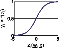
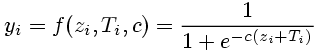
This sigmoid function can be configured with two parameters: T_i describes the shift of the function with the absolute value -T_i; the parameter c is a measure for the steepness. Given that c is larger than zero, the function is on the whole domain monotonically increasing, continuous and differentiable. For this reason, it is particularly important for networks applying backpropagation algorithms. For larger values of c the fermi function approximates a heaviside function.

(11)

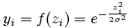
The maximal function value of a gauss function is found for zero activation. The function is even: f(-x)=f(x). The function value is decreasing with increasing absolute value of activation. This decrease can be controlled by the parameter Σ; larger values of Σ result in a decrease of function values with increasing distance from maximum (the function becomes 'broader').

(12)

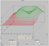
The simulation computes and visualizes the output of a neuron for different activation functions and output functions. The neuron receives two-dimensional inputs with the components x₁ and x₀ in the interval [0,1]. The weights are indicated as w₁ and w₀. Additionally, a 'bias' is provided.

The diagram shows the netoutput for 21x21 equidistantly distributed inputs.

Different activation and output functions can be selected in the boxes below the diagram left and right, respectively. Depending on the selected functions, different parameters can be changed. The slider on the right side of the diagram shifts a virtual separation plane parallel to plane x₁-x₀. Red: outputs below the separation plane. Green: outputs above the separation plane.

Separation plane for XOR-function

• Start Simulation
• Choose activation "dotproduct"
• Choose output "ramp"
• Choose Parameter: w₀=0, w₁=1, Bias=1
• Choose Threshold T₁=0.3; T₂=0.8

Open Simulation

• 1. Set weights to w₀=0.5 und w₁=-0.5! Choose "dot product" as activation function!
• a) Set output function to "linear"! How does the straight line run that is defined by the weights? Choose as output function "step" with the threshold value T=0 and verify your results!
• b) Increase threshold value T to 0.2! How does the line that is defined by the weights runs now? Explain the difference to exercise 1a!
• c) Choose "sigmoidal" as output function and determine the parameter T_i ("shift") as well as c ("steepness") in a way that you obtain the results in exercise 1b. Explain your results!
• d) Choose "gaussian" as output function with Σ=0.1 ! Does the combination of the gaussian function with the dot product function make sense? Explain!
• 2. Set both weights to 0.5 and the activation function to "Euclidian distance"!
• a) Choose "gaussian" as activation function with Σ=0.1! Compare your results to exercise 1d! What difference does it make?
• b) Choose "sigmoidal" as output function with the parameters T_i=-0.1 ("shift") and c=25 ("steepness")! Compare your results to exercise 2a! Which output function ("sigmoidal" or "gaussian") is optimally applied in a network that shall produce a maximum similarity between input vector and output vector?
• c) Find a way to rebuild the plot from exercise 2b with a ramp function as output function! Name the values of the thresholds T₁ and T₂?
• 3. Set both weights to 0.5 and use "step" as output function! Compare the output for "euclidian distance", "manhattan distance", "max distance" and "min distance" as activation functions. Vary the threshold T in the interval [0.2,0.4]! Name the geometrical forms that describe the subspaces of the input space, where the neuron produces zero output? Why do the subspaces show the specific form?

• Title: Transfer Functions Simulation
• Description: This simulation on transfer functions visualizes the input-output relation of an artificial neuron for a two dimensional input matrix in a threedimensional diagram. Different activation functions and output functions can be chosen, several parameters such as weights and thresholds can be varied.
• Language: English
• Author: Klaus Debes
• Contributors: Alexander Koenig, Horst-Micael Gross
• Affiliation: Department of Neuroinformatics and Cognitive Robotics, Technical University Ilmenau, Germany
• Creator: Klaus Debes
• Publisher: Author
• Source: Author
• Rights: Author

• Application context: bachelor, master, graduate
• Application setting: online, single-user, talk, course
• Instructional use: A theoretical introduction into artificial neural networks and/or system theory is recommended. Time (min.) 90
• Resource type: simulation, diagram
• Application objective: Designed for an introductory course in neuroinformatics for demonstrating the input-output behaviour of artificial neurons as it depends on different activation and output functions.

• Required applications: any java-ready browser
• Required platform: JAVA Virtual Machine
• Requirements: JAVA Virtual Machine
• Archive: transfer_functions.zip
• Target-type: Applet (Java)
• Target: ../applets/AppletSeparationPlane_wot.html

• 1. Start the simulation at the link "Transfer Function Simulation" in the article.
• 2a. Alternatively, download archive from http://www.brains-minds-media.org
• 2b. Unpack in an directory of your choice.
• 2c. Move to the chosen folder
• 2d. Start the simulation by calling "AppletSeparationPlane_wot.html"

• 1. Start Simulation
• 2. Choose activation "dotproduct"
• 3. Choose output "ramp"
• 4. Choose Parameter w0=0, w1=1, Bias=1
• 5. Choose Threshold T1=0.3; T2=0.8