
Document Actions
Simbrain: A visual framework for neural network analysis and education
UC Merced, School of Social Sciences, Humanities, and Arts; Center for Computational Biology, P.O. Box 2039Merced, CA 95344, USA
urn:nbn:de:0009-3-14114
Abstract: Simbrain is a visually-oriented framework for building and analyzing neural networks. It emphasizes the analysis of networks which control agents embedded in virtual environments, and visualization of the structures which occur in the high dimensional state spaces of these networks. The program was originally intended to facilitate analysis of representational processes in embodied agents, however it is also well suited to teaching neural networks concepts to a broader audience than is traditional for neural networks courses. Simbrain was used to teach a course at a new university, UC Merced, in its inaugural year. Experiences from the course and sample lessons are provided.
Keywords: Neural Networks, Visualization, Dimensionality Reduction, Virtual Reality, Simulation, Neural Networks Education
In the past ten years an impressive array of neural network simulators, many of them free and open source, have emerged. In what follows I describe one of these simulators, Simbrain ( http://www.simbrain.net ), which I began to develop while writing my dissertation on philosophy and cognitive science in the 1990's. Simbrain is distinguished by its particular set of emphases: ease of use (e.g. user can download, run, and within seconds interact with a running network using a familiar interface), ability to create networks of arbitrary topology, use of realistic environments and virtual worlds, graphical representation of network state spaces using a variety of projection techniques, and use of open source java components and object oriented design principles to facilitate easy extension and evolution of the code. Other frameworks emphasize some of these features (and others not emphasized by Simbrain), but none emphasize this particular collection of features in the same way.
In what follows, I lay out Simbrain's emphases relative to the history of its development, describe its architecture and features, and show how it was used in a specific educational setting. I argue that the tool has at least two main benefits currently. First, it provides an ability to visualize representational processes in embodied agents, which may provide a new way of thinking about the relation between biological and cognitive process. Second, I argue that this framework is well suited to teaching neural networks concepts both to traditional and non-traditional students of the topic, based on experiences teaching a course with it in 2007. Sample lessons from the course are provided. In the conclusion I consider other potential values of this type of framework. Throughout the emphasis is on Simbrain 2.0, the current release, though features planned for 3.0, which is under active development, are noted. Many 3.0 features can be tested by obtaining the latest developer snapshot from http://www.simbrain.net/trac .
To better understand the purpose and overall philosophy of Simbrain, as well as what distinguishes it from similar packages, it helps to describe the motives which led me to create it. My first interest in neural networks came while I was an undergraduate at UC Berkeley in the early 1990's, majoring in philosophy. I was taking courses with John Searle and Hubert Dreyfus, both of whom had philosophically oriented arguments against artificial intelligence, based on their respective theories about the mind. Both had directed their arguments initially against classical rule based systems, but had developed variants of their arguments when connectionist networks became prominent in the late 1980's. I was captivated by these discussions, and took the position that regardless of whether computers could think, (1) brains are the causal basis of mental processes and thinking, (2) computer models of the brain allow researchers to study the dynamics of neural activity in ways not possible by direct empirical observation, and therefore (3) computer models of the brain can shed light on the dynamics of mental processes and thinking.
In developing these ideas, I was led to study the philosopher Edmund Husserl, and was struck by a series of parallels between his 100-year old theory of mind and current connectionist theories of mind and brain. The parallels were especially striking given that the two theories had developed independently. Husserl had said that the mind could be understood relative to a vast space of possible mental states, and that mental processes could be understood in terms of law-governed structures in that space. Connectionists were saying that the brain could be understood relative to a vast space of possible brain states, and that brain processes could be understood in terms of law governed structures in that space. So we had spaces of mental states and brain states, each governed by its own laws. Showing how these two spaces and the rules governing them relate to each other became my philosophical project. I subsequently studied Husserl with David Smith at UC Irvine, and neuro-philosophy with Paul and Patricia Churchland at UC San Diego. Today I continue to work on this project at UC Merced, the tenth and newest campus of the UC System, where I have been able to work closely with faculty in cognitive science.
Early in this process I realized that I would have to develop my own simulations. I wanted to visualize the state space dynamics of neural networks attached to simulated environments. None of the freely available packages available at the time could do this. Thus I began work on what is now Simbrain. In the remainder of this section I describe the program's purposes in terms of the requirements that my philosophical interests generated.
My first requirement was that the program be visual and easy to use. I wanted to be able to observe network dynamics over time. As I began my work some programs emerged which offered visualization, but they were typically focused on particular classes of network. Also, I had specific intuitions about how the user interface should work, based on my experience with standard vector-based drawing programs. I wanted to be able to create neurons and groups of neurons, copy and paste them, lasso select them, zoom in on them, etc. I wanted to be able to quickly mock up networks and experiment with them. A related issue was that I wanted to be able to easily run the program, with minimal requirements in terms of installation: the user experience I was after was one where a user would download, double click, and within seconds be interacting with a neural network.
Second, I wanted to be able to create networks with arbitrary structure. I wanted to be able to take Hopfield networks, competitive networks, free-floating assemblages of neurons, etc. and wire them together easily and quickly. As we will see below, providing this level of generality posed a number of challenges.
Third, I wanted to study processes where an agent was exposed to an object from multiple perspectives over time (Husserl often describes processes of experiencing the same object from multiple perspectives). This could be modeled using hand-coded sequences of vector inputs representing successive appearances of an object, but I wanted to have some ability to study these processes in a more flexible manner. I wanted to be able to actually manipulate an agent in a simulated or "virtual" world, changing its position with respect to various objects, observing the resulting patterns in its state space. Thus it was important that some form of simulated world be included with the program
A fourth, crucial aspect of the project was that I wanted to be able to visualize patterns in the state space of the neural network. It is common in philosophical discussions of neural networks to refer to patterns appearing in state space, e.g. activation space or weight space. Perhaps more than any other philosopher, Paul Churchland has emphasized the significance of this approach for traditional philosophical problems. As he put it:
The basic idea… is that the brain represents various aspects of reality by a position in a suitable state-space; and the brain performs computations on such representations by means of general coordinate transformations from one state-space to another… The theory is entirely accessible-indeed, in its simplest form [under 3 dimensions] it is visually accessible ( 1986, p. 280 ).
To illustrate these ideas Churchland, following standard practice in philosophy as well as cognitive science, uses 2- and 3 dimensional examples, or other diagrams based on projections of high dimensional data to 2 or 3 dimensions. In researching the issue I realized that there were numerous ways to project high dimensional data to lower dimensions, and thereby to make these ideas accessible even in their more complex form. So, in line with my general emphasis on real-time experimentation and intuitive interfaces, I worked to build a mechanism for producing these projections in real-time, and for comparing them. I teamed up with a mathematician , Scott Hotton, to build a mechanism for using one of several methods for projecting data from arbitrary dimensions to two dimensions. We validated the program using well understood properties of other high dimensional objects (e.g. 4 dimensional cubes and tetrahedra, boquets of circles, and the projective plane), and released it as a separate product (see http://hisee.sourceforge.net/ ).
Finally, I wanted the code itself be easy to obtain, use and extend. Java was a natural choice, because of its extensive built in library and cross-platform compatibility. Open source was also a natural decision, in order to encourage a community of developers to contribute to and thereby evolve the program. Also, it was important that well known object oriented patterns and principles should be used and that the API (application programmer interface) should be clean and simple to work with. Towards these ends, a web site using graphically intuitive software was set up to facilitate discussion of and modification of the code ( http://www.simbrain.net/trac ), and we have pursued an ongoing cycle of reviewing and "refactoring" (redesigning) the code in order to improve its overall design, and hence its stability, extensibility, and ease of use. Existing open source libraries have been used as much as possible. The hope is that Simbrain will be able to leverage improvements made to the java libraries (java recently became open source) and to other related open source programs as they develop.
The cumulative result generated by these requirements is a program which allows the user to build a wide variety of networks, embed them in environments, and to study the resulting dynamics by looking at projected representations of state space. Moreover, the code should be clean enough to facilitate the introduction of new types of network, world, and visualization over time, by the efforts of the open source community.
To run Simbrain download it from http://www.simbrain.net/Downloads/downloads_main.html , and double click on the Simbrain.jar file. You will need to have the java runtime environment installed. Tutorial type information is minimal here; for a tutorial on creating simple simulations, see ( http://www.simbrain.net/Documentation/docs/Pages/QuickStart.html ).
When the program is run a "workspace" opens (see figure 1), which is a collection of components which can be coupled together in various ways. This is visible as a "desktop," and each component exists as a window in this desktop. Menus in the upper left corner of the workspace allow users to add new components to the desktop and to open and save collections of components. Currently there are three kinds of workspace component: networks, virtual worlds, and gauges, which correspond to neural networks, simulated environments which those network can be attached to, and devices which allow for the visualization of structures in a high dimensional space. Users can add arbitrarily many components to Simbrain. Simbrain opens with a default workspace, and a set of built in workspaces are also provided. To explore these, select "open workspace" from the File menu, and peruse the directories. Collections of components can be saved and reopened.
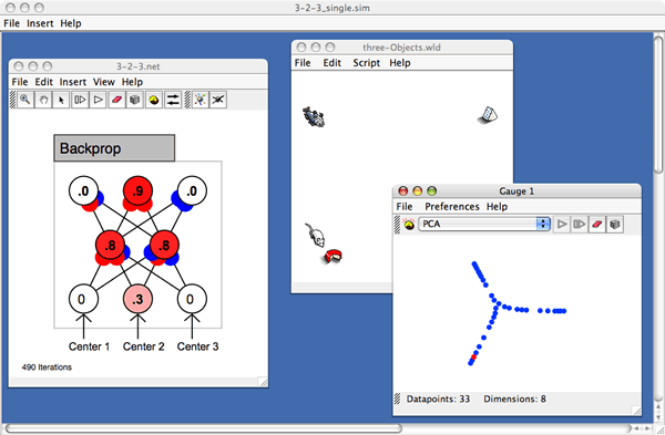
Figure 1: The Simbrain Workspace
The architecture supporting workspace interactions is being redesigned for the 3.0 release, in order to support more complex environments and component interactions (including distributed environments involving multiple instances of Simbrain communicating over the internet). In the remainder of this section, the three currently available types of workspace component are described in more detail.
Network components, which display neural networks, are the primary Simbrain component (see figure 2). The main design goals of the network component, as noted above, were to make use of familiar interface elements, to allow users to quickly build networks with arbitrary topologies (i.e., networks merging a wide variety of neuron types, including spiking neurons, as well as different network types), and to allow the code to be easily extended. We will see that the generality built in to the network component required that a number of special features be added, including the concept of a "sub-network," and, for future releases, the concept of a logical group of neurons and / or synapses. We will also see that many concepts associated with building networks are such that they can be extended in a modular fashion: neurons, synapses, sub-networks, methods for creating synapses, and methods for laying out groups neurons are among the functions that can currently be customized by the user.
Networks are displayed using colored circles and lines. The colored circles with numbers in the middle represent model neurons (henceforth "nodes" or simply "neurons"). The numbers inside the neurons typically represent activation, though what "activation" means varies, depending on the neuron type. The number is rounded though an exact value can be obtained by lingering over a neuron for a tooltip or double clicking on it. The color of a neuron represents its activation: shades of red for values greater than zero, with more intense values closer to the neuron's upper bound, and shades of blue for values less than zero, with more intense values closer to the neuron's lower bound. Zero activation is represented by white. These color conventions can be customized by the user.
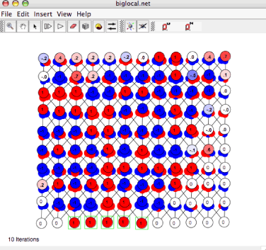
Figure 2: A Simbrain Network
The lines between model neurons represent connections between neurons. The smaller blue and red discs at the ends of these lines represent synapses (henceforth "weights" or simply "synapses"). The size of the disks is proportional to how far the synaptic strength is between 0 and its upper or lower bound. The exact strength can be determined by lingering over a synapse or double clicking on it. The color of a synapse represents whether the strength is greater than 0 (red) less than 0 (blue), or equal to 0, grey. The last case represents the absence of a weight. These conventions can also be adjusted in the preference dialog. Learning in a neural network is visualized by incremental changes in the size of these weights. As the network runs an iteration number is shown. Flows of color through the network show activation flow, and changing weight diameters depict incremental synaptic adjustment.
Groups of neurons and / or synapses are selected by dragging the mouse to "lasso them." Right-click context menus are sensitive to the object which is clicked on, and show appropriate actions. Double clicking calls up a property dialog which allows an object or group of objects to be edited. Shift selection and lasso-unselect allow for large groups of neurons and synapses to be specifically selected. In this way large groups of elements can be edited. Neurons and synapses can also be copied and pasted. The network as whole is written using an open source "zoomable user interface" library (piccolo: http://www.cs.umd.edu/hcil/jazz ) which makes it easy to zoom in on and navigate complex networks. "Semantic zooming" allows the network representation to change depending on the level of zoom (e.g. when zoomed way out only high level properties of the network are shown), though this has not been fully utilized with the current release.
These features allow users to rapidly create and edit neural networks. A user can create a line of neurons and copy-paste this line to quickly create a large group of neurons. The user can then select various subsets of these neurons to change their properties. Neurons can be connected using various commands, and the synapses produced can be lasso selected and edited in the same way neurons can. The resulting networks can be analyzed immediately, by running the network. Activation can be injected, weights can be randomized, and so forth, by lassoing relevant elements and pressing the randomization button or the up /down arrow keys. For more, see lesson 1 below, or the quick start ( http://www.simbrain.net/Documentation/docs/Pages/QuickStart.html ). In version 3.0 the process of building and editing networks is even easier. Smart copy / paste allows networks to be "grown" out based on previous pastes, and a connection framework has been added which allows large groups of neurons to be connected together in a few keystrokes using one of a set of pre-defined algorithms or a custom algorithm designed by the user.
In 2.0 there are 16 neuron types, each with its own update rule. The property dialog for neurons or groups of neurons is shown in figure 3.
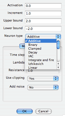
Figure 3: The Neuron Properties Dialog
The top part of the dialog shows properties that are common to all neurons. In the middle is a drop down box that allows the user to change the type of neuron. As the neuron type is changed a section of the dialog with properties specific to that neuron type appears. In the underlying code, it is relatively straightforward to add new neuron types, by creating a subclass of an abstract Neuron class, and by performing straightforward tasks to wire the graphical interface together. Adding neuron and synapse types is documented on the developer wiki: http://www.simbrain.net/trac/wiki/AddNeurons .
The same set of features applies to the model synapses. Individual synapses or groups of synapses can be interacted with via lasso selection, modified using a right click context menu, and edited using a similar dialog, and it is easy to add new synapse types to the code.
Creating and editing predefined neuron or synapse types from a menu of choices allows any generic type of network to be built, simply by creating neurons, changing their types, and wiring them together. This can actually be done as the network runs (e.g. the type and parameter of a subset of neurons can be changed) resulting in a dynamic way of understanding effects of different types of learning rule. However, this level of generality poses special challenges that had to be addressed. To understand these challenges, it is useful to consider the way network update works.
Simbrain networks contain a list of neurons and a list of weights. Each time the network is updated the program iterates through each of these lists, and calls an update function on each neuron and each synapse. This allows for generality, since all that is required of a neuron and synapse is that they have an update function and a few common properties, including an activation value, upper bound, and lower bound. Neurons have access to all the neurons they are connected to, so their update functions can make use of information available via their local connections to other neurons, and similarly for synapses, which have access to their source and target neurons. Since the order in which neurons and synapses are updated cannot be set by the user, a buffering system is used so that update order does not matter (neuron activation values are placed in a buffer at the beginning of each update cycle, and applied at the end of the cycle). This system allows for the generality characteristic of Simbrain networks, but poses several problems.
First, in many cases the way a network is updated requires that neurons or synapses have information that is not locally available. For example, backpropagation requires that synapses know about error values computed outside the network altogether (by comparing actual and desired values at the output layer). Winner-take-all networks must query every neuron in some subset of neurons to see which is receiving the most input. Some networks require forms of update incompatible with buffering (e.g., Hopfield 1984 ). None of these networks can be implemented using the update method just described.
To address these problems, the concept of a subnetwork was introduced with Simbrain 2.0. A subnetwork is itself a network object in the underlying code, with a list of neurons, synapses, and in some cases, further subnetworks. However, a subnetwork has its own custom update function. A sample subnetwork is shown in figure 4.
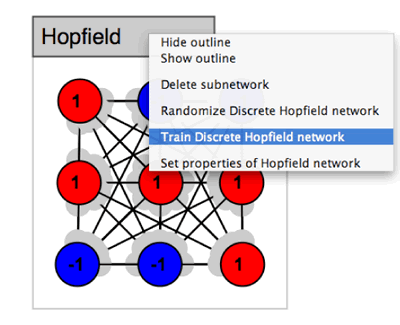
Figure 4: A Sub-Network and Context Menu
The subnetwork shown in figure 4 is a Hopfield network. The grey outlined tab at the upper left serves as an interaction point for the subnetwork. The tab can be used to move the network relative to other Simbrain components, can be double clicked on to reveal a properties dialog with properties specific to that subnetwork type, and can be right clicked on to reveal a context menu (show in figure 4). For example, in the Hopfield network shown there is a special randomization function that randomizes its weights so that they remain symmetric. As with neurons and synapses, users create new network types simply by extending a base class and following directions on the developer wiki. When subnetworks are created, a dialog appears, which allows the user to set various features of the network. For most networks users can select how their neurons will be positioned. This layout can be customized by creating a custom extension of the layout class.
So, the overall structure of Simbrain is that it contains a list of neurons, a list of weights, and also a list of subnetworks, each of which can contain its own weights, neurons and subnetworks. This defines a hierarchy of networks, with a root network at the top of the hierarchy (it is in this network that "free floating" neurons and synapses exist), and subnetworks below. This presents some complexities in the code (e.g. nodes at any level of the hierarchy can be connected by synapses, so that connections can span across layers of the hierarchy), but it does allow for the use of arbitrary network topologies.
A second issue raised by the generic nature of Simbrain networks concerned spiking neurons and spiking neural networks. The neuron types described above correspond to traditional connectionist models where activations represent firing rates or activation abstractly conceived. However, more realistic model neurons include discrete firing or "spiking" events which correspond to action potentials. Simbrain includes two types of spiking neurons: basic integrate and fire neurons and a more sophisticated model due to Eugene Izhikevich (2004) , which is general enough to capture many forms of spiking and bursting activity. A network of spiking neurons is shown in figure 5.
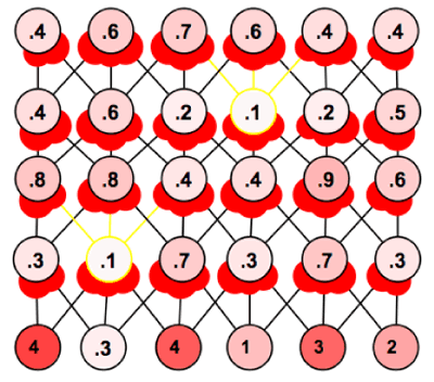
Figure 5: A Spiking Network
For spiking neurons, activation corresponds to something like voltage potential and firing events are represented by the boundary around the neuron and all outgoing connections changing to a color set by the user (yellow above, and by default).
The problem raised by incorporation of spiking neurons is that discrete spiking events must be translated into numerical values, in order to be used by subsequent neurons, which can use any arbitrary activation function (such problems do not normally arise since most simulations do not merge rate based and spiking model neurons). For example, most activation functions make use of a net input or weighted input term, which is computed by taking the sum of incoming activations times weights (the dot product of an incoming activation vector and weight vector). However, weighted inputs computed in this way lose the information associated with a spike. In order to address the problem, we adapt a method reviewed in ( Dayan and Abbot 2001 ), whereby spikes are associated with spike response functions which convert discrete spiking events into pulses of activation. Users can choose from several spike response functions and adjust their parameters. As with other Simbrain objects, it is relatively easy to add new spike response functions.
An additional problem involves the merging of model neurons whose activation functions are based on simple iteration with those based on numerical integration of a differential equation. We call these "discrete" and "continuous" neurons, respectively. Continuous neurons are associated with a global time-step parameter, which is used whenever differential equations are numerically integrated in Simbrain. When a continuous neuron or synapse is used, an iteration of the network represents an interval of time equals to the time-step. This is signified in the interface by displaying network iterations in seconds. Discrete neurons use simple iteration, so that time is simply thought of as number of iterations. If there are no continuous neurons or synapses then the network display shows current time using an integer number that simply represents number of iterations thus far. Again we have an issue of merging: what to do when simulations use a mixture of discrete and continuous elements? The solution used in Simbrain is as follows. If there is one or more continuous neuron or synapse in a simulation, then those elements are updated using the global time-step parameter. At each time-step, all the discrete elements are updated as well. To show that the time-step parameter is being used, network iterations are shown in seconds.
One additional issue to be addressed with the 3.0 release is that in some cases it is useful to have control over the order in which nodes and subnetworks are updated. Sometimes, in fact, an extremely fine grain of control will be desired, whereby, for example, neurons stop firing after some equilibrium is reached, or some other workspace component has entered a particular state or run for some specific length of time. To address these issues users are able to choose an update method in the 3.0 release. One of these, priority-based, allows the user to associate a priority value with each neuron and subnetwork. This takes away issues involved with buffering and gives control over update method to the user. Another, script-based update, allows the user to associate a custom script with a network which is run each time the network is updated, which provides the kind of control described above.
Another issue being addressed in the 3.0 release is that, even with neurons, synapses, and a hierarchy of subnetworks, there are forms of network dynamics that still cannot be captured. In particular, it is sometimes useful to apply a rule to a collection of networks, neurons, and synapses which does not respect the boundaries of a particular subnetwork. For example, we may want to implement a pruning rule, whereby some subset of weights in a network are checked every iteration (or nth iteration). These weights may span all levels of the subnetwork hierarchy, so that it would be impossible to associate it with one subnetwork's update rule (moreover, we want the flexibility to do this for any subnetwork type, rather than tying it to some specific subnetwork type). To handle cases like this, the concept of a logical "group" is being developed, so that with each iteration, in addition to updating subnetworks, logical groups - each with their own custom update method - are updated as well.
The overall concept is that the user has a lot of flexibility in building networks, and in extending Simbrain. The following features can easily be added now: new neuron types, synapse types, subnetwork types, spike response functions, and layout types (which determine how groups of neurons are positioned). With 3.0, it will be possible to easily add new connection types (for creating sets of connections between neurons) and group types.
Simbrain worlds are simulated environments, which produce inputs to and accept outputs from nodes in one or more neural networks. The use of the term "world" is a reference to German philosophers who emphasize the role of the "surrounding world" or "lifeworld" in cognition, as well as a growing recognition in cognitive science and philosophy that the study of cognition must incorporate analysis of the bodies and environment within which brains are situated (see Clark and Chalmers 1998 ). As noted above, an early design goal of Simbrain was to be able to study the way environments interact with neural networks in a flexible way: to be able to study neural networks insofar as they are embedded in agents which are embedded in complex, realistic, worlds.
It turns out that the underlying software design issues involved in creating a general framework for linking arbitrarily many neural networks with arbitrarily many environments is non-trivial. It is therefore being completely redesigned for 3.0. However, the 2.0 release does contain two types of world and allows for them to be connected together. The first ("Data world") is a simple table, which facilitates standard uses of environments for neural networks, where a series of input vectors are exposed to a network and corresponding outputs are recorded. The second, "Odor World", is more of a true virtual world; we focus on it here. More sophisticated worlds are being planned for the 3.0 release, and the way in which new worlds are developed and added to Simbrain is being simplified.
An OdorWorld window with four objects and one agent is shown in figure 6.
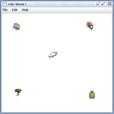
Figure 6: A Virtual World
The mouse in the center of figure 6 can be attached to a network in Simbrain. Network nodes can be attached to the mouse's sensors and effectors; in this way a neural network can model the response of the mouse to its environment and can control the mouse's movements.
Odor World is inspired by the olfactory system. Objects in the environment emit chemicals which bind to receptors inside a bank of tissue in the nose called the nasal epithelium. Different objects in the environment produce chemicals which have a characteristic impact on the receptors in this tissue ( Laurent 1999 ). Objects can therefore be associated with "smell vectors" which describe the pattern of activity they produce on an agent's nasal epithelium. The chemicals associated with objects diffuse in the atmosphere such that objects typically have a stronger impact on an agent when they are closer to it. This is modeled by scaling the smell vector by distance. When multiple objects are present to an agent overlapping patterns of activation are produced. This is modeled (somewhat inaccurately) by simple vector addition; we take the smell vectors associated with flowers and cheese, in the example above, and add them together. Thus the total pattern of inputs to a creature's olfactory receptors is a sum of scaled smell vectors; what an agent smells depends on what objects are within smelling distance and how far away these objects are. Though the model is based on smell it can be thought of in more general terms as a simple way of modeling distance based interactions with objects. Smell vectors are more generally "stimulus vectors" which describe that object's impact on an arbitrary bank of sensory receptors.
A node in a neural network can be attached to an agent (for example, the mouse in figure 6) by right-clicking on the node and following out a string of submenus which allow the user to choose a world, an agent in that world, and finally a particular "receptor" or "motor command" associated with that agent. When nodes are attached to receptors they become "input nodes" (this is signified by an arrow pointing in to that node). When nodes are attached to motor commands they become "output nodes" (this is signified by an arrow pointing out of that node).
Input nodes are associated with particular receptors on an agent. For example, an input neuron associated with a cheese receptor will be active when the associated agent is near a piece of cheese (in terms of stimulus vectors, receptors are associated with components in a sum of scaled stimulus vectors). How active the input neuron is is based on how far the receptor is from the relevant object. The way the receptors behave can be controlled by double clicking on objects and the agent. By double clicking on an object (e.g. the cheese or the flower in figure 6) its stimulus vector can be edited, the form of distance based scaling can be modified, and noise can be added. For example, we can specify that swiss cheese cause receptor 2 to be extremely active when the agent is nearby, and that its impact will diminish linearly by distance. By double clicking on the agent (the mouse in figure 6) the location of its smell receptors can be edited. This is important when an agent has to be sensitive to the relative location of objects, e.g. if it has to know that an object is to its left rather than its right.
Output nodes are associated with "output commands," which are essentially the motor controls of the agent. When coupling a neuron to an agent, one can choose between two styles of movement: relative movement, and absolute movement. Relative movements are motor commands that tell the agent how to move relative to its current orientation: e.g. move forward or to the right. Absolute movements tell the agent to move in directions that are independent of its orientation, such as move to the north or to the south-west. All movements are scaled based on the activity of the coupled neuron and a fixed movement factor (one for moving straight, one for turning). The larger the activation, the faster the agent. Odor World also provides mechanisms for drawing walls (though this is currently relatively simplistic) and for allowing objects to disappear and reappear.
Using these tools one can connect neural networks with agents in a simple virtual world. To get an intuitive sense of how this works open the simulation sims > two-agents (the default simulation when initially running Simbrain), and press play in one or both of the networks. You can also manually move objects or agents in the world around. Also see the second lesson below.
Plotting and charting capacities are essential to any neural network simulator. As noted above, one specific type of visualization was emphasized in the initial Simbrain design: projection of structures in high dimensional spaces to two dimensions. This is the gauge component, or "high dimensional visualizer." A screenshot of a high dimensional visualizer is shown in figure 7.
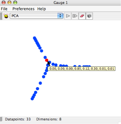
Figure 7: A High Dimensional Visualizer
Each blue dot in the visualizer represents a point in an n-dimensional space (i.e., a list of numbers), a vector with n components, which has been projected into two dimensions. The components of these vectors can come from neural activations or synapses in any combinations (so that activation spaces, weight spaces, and combinations of the two can be visualized), and in 3.0 they can arise from any arbitrary workspace parameters. Typically these correspond to all the neural activations of a neural network or one layer of a neural network, so that each blue dot represents a total activation state of a network. The status bar at the bottom shows how many points are currently plotted and what the dimension of the space these points live in is. The blue dots corresponds to states that have occurred previously, and the red dot corresponds to the current state. Lingering over any point presents a tool tip which shows the actual high dimensional vector the point represents. In the example above, the dots represent states of an 8-node neural network, whose current neural activations are, as the tooltip shows, (0, 0, 0, 0, .85, .12, .30, .01, .01). 33 unique states have occurred in this network thus far.
The representation in the visualizer which is attached to the nodes of a neural network present us with a kind of visual history of the states that have occurred in a neural network up to the present point. When running a neural network with a visualizer attached one initially sees these points populate the gauge. Over time, as states that previously occurred recur, a stable pattern develops which shows the set of representations that occur for that network in its current environment. The agent's current state relative to this set of representations is visualized as a red dot that moves within the pattern that has formed.
In the example shown above in figure 7, the gauge represents states of a network in an environment with three objects. 33 network states, each representing a different position of the agent with respect to these objects, have occurred thus far. These representations form a "boquet of arcs," a collection of arcs joined at a single point. Each arc represents one of the objects, the center where the three arcs attach represent absence of any object, and the end-points of the arcs correspond to maximal exposure to one of the objects. As the agent moves towards one of the objects, the red dot moves from the origin out towards one of these ends. Thus, the combination of the gauge and the world allows the user to study the topological and geometric structure of its representation of its environment, a significant capacity for the study of mental representation. To try this simulation open the workspace file sims > bp > 3-2-3_single.sim, create a gauge, and move the agent around the objects.
The gauge allows users to compare the way a high dimensional structure looks under different projections. Three are provided: coordinate, PCA, and Sammon. By comparing the way different projection algorithms present a dataset users can gain qualitative understanding of high-dimensional structures. Consider efforts to project a globe to two dimensions. Even though each projection introduces its own distortions, by comparing them one gets a sense of the three-dimensional structure of our world. Let us consider each of the projection methods currently provided. Coordinate Projection is the simplest of the three, and is best explained by example. If one has a list of datapoints with 40 components each, coordinate projection to two-dimensions simply ignores all but two of these components, which are then used to display the data in two-space. PCA builds on coordinate projection by making use of the "principal axes" of the dataset. The principal axes of an object are the directions in space about which the object is most balanced or evenly spaced. PCA selects the two principal axes along which the dataset is the most spread out and projects the data onto these two axes. The Sammon map is an iterative technique for making interpoint distances in the low-dimensional projection as close as possible to the interpoint distances in the high-dimensional object ( Sammon 1969 ). Two points close together in the high-dimensional space should appear close together in the projection, while two points far apart in the high dimensional space should appear far apart in the projection. When using the Sammon map a play and iterate button are highlighted which allow the user to start and stop the iteration process.
In some cases it is useful to be able to add new points to an existing dataset without running the projection method on the whole dataset again (since this is computation intensive). Methods exist for quickly adding new data points based on data that have already been projected. These methods work best when a certain amount of data has already been collected and projected using, for example, PCA or the Sammon map. These methods can be accessed in the visualizer via the preferences menu.
Beyond high dimensional visualization, there is no charting capacity in Simbrain 2.0, though as part of the 3.0 an open source package will be used to add more standard forms of charting.
Simbrain was developed on the basis of my specific interest in observing the state space dynamics of neural networks embedded in realistic environments. The resulting emphases on visualization, ease of use, and virtual environments lend themselves naturally to education. In fact, this kind of framework makes it possible to convey many ideas relating to neural networks to students without formal training in mathematics. There is value in teaching these ideas to a broad audience. For example, psychology students are often not required to take linear algebra or even calculus, but neural networks models have obvious relevance to psychology. Being a faculty at a new university, UC Merced, provided an excellent framework for testing the idea that neural networks as models of cognitive processes could be taught to students with minimal background in advanced mathematics.
UC Merced is the tenth, newest campus of the UC System, and was opened to undergraduates in Fall 2005. The university is committed to the use of open source, computer facilitated education, and to innovative pedagogy. The university is also interested in making connections with local community colleges in California's central valley, where transfer rates to universities have traditionally been lower than those in the state as a whole. With these consideration in mind I developed a course around Simbrain (with plans to develop specific modules based on this course which can be used in community colleges and high schools).
The course was taught in Spring 2006, and was based on on-line content written for the course, which will be released at a future date under an open content license, so that users will be able to change and adapt the course to their specific needs. The course was called "Neural networks in cognitive science," and its purpose was to introduce students to basic concepts of neural network theory as well as their application to modeling biological and cognitive processes. This was the first neural networks course ever taught at UC Merced. There were 13 students in the course, some of whom had no calculus background, and none of whom had taken linear algebra. The students came from a broad array of majors, including psychology, economics, cognitive science, and business management. Each week students read 10-20 pages of material, and participated in a lab, in which they created simple models in Simbrain and answered questions relating to these models.
The course as a whole consisted of 25 lessons and 10 labs, and was broken in to three parts: (1) Fundamental Concepts, (2) Architectures and Learning Rules, and (3) Applications to Biology and Psychology. These lessons and labs were designed to be semi-autonomous, so that they could be adapted to individual lessons used by others in other educational settings, e.g. community college or high school courses (again, the lessons will be released under an open content license so that the material can be adapted to the needs of particular learning environments).
Four lessons are included in the appendix, which are adapted from lessons and labs used in the course. These lessons utilize all the Simbrain components - networks, virtual worlds, and high dimensional visualizers – to help students develop an understanding of the basic concepts of neural networks as they apply to biology and cognitive science.
The first lab introduces students to the basic visual semantics of the Simbrain interface, and provides a first-pass, intuitive understanding of the way neural networks function, in particular, how flows of activation are channeled through the nodes of a network, and how these flows are determined both by patterns of sensory input and by the nature of the weighted connections between nodes. In the lab, students change sensory inputs, as well as weights between nodes, to see how this affects the overall activity of the network. Students were also shown how to give the weights a learning rule, and in this way could see how a network could change its response to stimuli on the basis of past activity. They could see weights get stronger or weaker and the impact this had on network activity. This made intuitively clear how weights are conceived as the substrate of learning in a neural network, and how learning can be understood in terms of changing response to a fixed sensory input.
The second lab shows how neural networks can be used to control the behavior of agents in a virtual environment. Students interacted with a network which models "hunger" or "desire" in a simulated agent in an Odor World component. The sensory inputs that were manipulated by hand in the first lesson now arise from sensory receptors of an agent in a virtual environment, which detects the presence of a fish. This gives students a sense of the way network activity arises and changes based on an agent's position in an environment. Moreover, whereas in the first simulation this activity propagated through the network and dissipated, in this simulation network activity controls the agent's behavior. Thus, the way nodes, weights, inputs, and outputs can work together to coordinate intelligent behavior is made intuitively clear.
The third lesson below (not the third lesson for the students) begins to introduce some of the more abstract concepts of neural network theory, in particular, the use of dynamical systems theory to analyze network behavior. While previous lessons use various types of feed-forward network, this lesson uses recurrent networks which display more complex forms of dynamical activity, in particular, periodic orbits, attractors, and repellors. The students were able to understand these dynamical concepts by building recurrent networks themselves, directly manipulating their activity, and observing the projection of this activity in the high dimensional visualizer. For example, the period of a limit cycle could be observed by iterating the network, and tracking the current point in the gauge; a period-4 limit cycle would go through four different points in the gauge until repeating. In this way basic dynamical concepts, as well as their application to neural networks, could be immediately and intuitively understood.
Thus far students have used all the central components of Simbrain: the networks, virtual world, and gauge. The fourth lesson included below shows how these components could be linked together to describe a neural network model of a cognitive phenomenon. The lesson focuses on cases of perceptual ambiguity, where subjects perceive the same stimulus in multiple ways. Students were asked to gather simple psychological data, in particular, timing of perceptual shifts relative to an ambiguous figure, and were shown how this data could be modeled using a biologically plausible model, in this case a 2-node winner take all network modeling firing rate as well as spike frequency adaptation. The dynamics of the network could be directly observed: one neuron, supporting one of the perceptual interpretations, would achieve peak activation, and thereby suppress the other. The presence of adaptation, however, meant that this activation would die out during sustained activation, allowing the other neuron to win the competition until its own adaptation kicked in. This oscillation of winners and adaptation produced a cycle of activity in the two nodes which could be visualized as a cycle in the gauge. Students were asked to adjust parameters on the model so that it would fit the rate at which they observed themselves shifting between perceptual interpretations. In this way students saw in a very simple framework how a biological model could be fit to psychological data to provide a hypothetical explanation. Moreover, the value of visualizing dynamical processes in producing this explanation was made clear.
These four lessons give a sense of the kind of progression that was achieved in the course; from basic concepts to a sense of how these concepts could be used to model biological and cognitive phenomena, as well as their interrelation. Other lessons addressed classical and operant conditioning, graceful degradation, visual search, and models of the retina. Although the course was focused on students without background in calculus or linear algebra, relevant concepts were still taught, e.g. the use of gradient descent in backpropogation and the use of feature vectors in competitive learning. The overall intent is that the basic components of Simbrain and the course can be adapted to a variety of audiences, including students with and without mathematics training.
Although the effectiveness of the course was not studied in a systematic way, observation and informal feedback (obtained via an email questionnaire) suggest that the use of Simbrain in conjunction with labs and lectures was effective. The students got up to speed building simple networks within the first hour of the first lab, and completed all labs with little difficulty. Concept acquisition was facilitated by seeing neural network concepts "in action" and being able to "play" with networks interactively. As one student said, "I wouldn't have been able to grasp some of the concepts if it hadn't been for Simbrain. It really helped to be able to see the different mechanisms and play with them yourself." Or, as another student put it:
Had it not been for Simbrain… I'm not sure I would have understood the concepts as well as I did. It was very helpful to put the concepts we learned in class into a visual model that I created. Just reading and going to lecture might help me memorize the material, but using Simbrain in conjunction with the lectures and readings allowed me to learn the material.
It is not clear how Simbrain compares with other packages in this regard, though in a previous semester I had taught similar ideas to a small group of students using a commercial textbook and the software packaged with it, which was not visually intuitive. The students clearly had a harder time grasping basic concepts in that course than in the course based on Simbrain, though again, the comparison was not carried out in a systematic way.
Simbrain shows how by combining three existing forms of technology - neural networks, virtual worlds, and high dimensional visualization techniques - it becomes possible to see the topological and geometric structure of representational structures that occur in agents. I believe that this has tremendous potential in terms of understanding how the dynamics of cognition and consciounsess arise from the underlying dynamics of neural activity in the brain. Indeed, I believe that we have only begun to appreciate the significance of the structures that occur in the high dimensional state spaces of embodied agents. With more powerful computers, optimization and continued development of the underlying code, and elaboration of relevant theory (see, e.g. Hotton and Yoshimi, in preparation ) I think that we will be able to visualize cognitive processes in ways that could hardly be imagined a generation ago.
As we have seen, these motives produced a tool which is well suited to educational application as well. Courses in neural networks are typically taught to computer science and engineering students, or to cognitive science students who have satisfied calculus and linear algebra pre-requisites. However, the underlying principles of neural networks and their application to the study of biology and cognition are simple enough that a broad range of students - including high school students and even younger students who have not taken relevant mathematics courses - should be able to understand them, especially when the concepts are taught using visually intuitive and familiar interfaces. This is all the more important given the increasingly important role neural networks play in the sciences of mind, together with the fact that many psychology and cognitive science undergraduates are not required to take calculus or linear algebra.
One arena in which Simbrain has not been used is in conventional neural network research, in part because there are such high quality toolkits already available, in part because Simbrain is still being expanded. However, I do see these as areas where the tool can develop. 3.0 is being written in conjunction with several researchers towards that end. Backpropagation, reinforcement learning, and the Leabra framework are among the models being rewritten or introduced with the new release, with the hope that it will be possible to analyze these models in new ways using the features Simbrain offers.
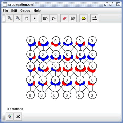
Lab: Propagation of Activity
For this example we will not assume any knowledge of the mathematics of neural networks. The goal is simply to get a sense of the way neural networks channel information, the impacts of changing inputs and weights on information flow in a neural network, and at a very broad level, the structure of learning as synaptic modification.
Begin by clearing the workspace, and opening a sample file:
-
In the Workspace, clear workspace using File > Clear Workspace from the main window.
-
Open a new network using File > New Network.
-
Open a network file using the menu File > Open.
-
Select lessons > propagation.xml.
Now try changing the bottom row of the neurons:
-
Select the bottom neurons using a lasso or, alternatively, select neurons individually by holding shift and clicking on each of the six bottom neurons. (These bottom neurons that are now selected can be thought of as input neurons.)
-
Randomize the neurons by pressing R or by pressing the random button (which looks like a die)
-
Iterate the network to see activation propagate through the network's nodes, by pressing either spacebar or the step button repeatedly. You can also press the play button.
-
Randomize the neurons again as described above and iterate the network through to see new network reactions.
-
Alternatively, try pressing the play button and then repeatedly randomizing the bottom row of neurons.
Next play with changing weights:
-
Be sure there is some activity (some color) in the bottom row of neurons.
-
Now select all synapses by pressing the W button or using Edit > Select > Select All Weights.
-
Randomize the weights using R or by clicking the random button above the network.
-
Propagate the network using spacebar or clicking the step button repeatedly until network propagation can no longer be seen.
-
Alternatively, press play and then repeatedly press the random button to see how this affects propagation of activity.
Finally, we modify the synapses so that they can change based on neural activity, which is how learning is modeled in neural networks:
-
Select all weights by pressing W or using the menu Edit > Select > Select All Weights.
-
Open the synapse dialog box by either double clicking on a synapse or using Edit > Set 64 Selected Synapses (if you "miss" you will have to reselect the synapses).
-
Using the drop down box, select Hebbian from the list of synapse types and set learning rate to 0.1 (or, if you will be using the play button, try .01 or even .001--the smaller the momentum the slower changes happen).
-
Now select the bottom row of neurons as described above and randomize the neurons.
-
Propagate activity using the spacebar, clicking on the step button repeatedly, or pressing play.
-
Observe changes in the sizes of weights as activity propagates.
-
Repeatedly randomize the neurons and observe changes in the weights.
-
You can also repeatedly randomize the weights and observe how they change.
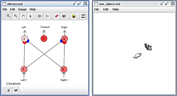
In this example we couple a neural network to a simple environment. The network below controls the mouse on the right. The mouse is similar to a vehicle described by the neuroscientist Valentino Braitenberg, in his book, Vehicles ( Braitenberg 1984 ). The vehicle occurs in chapter 2 of that book, and is described as being "aggressive," because it runs up to the thing it's attracted to as if it's attacking it. In this case the mouse is attracted to the fish.
Again begin by clearing the workspace and opening a sample file:
-
Clear the workspace by using File > Clear Workspace located in the workspace window.
-
Open a workspace using File > Open Workspace.
-
Select lessons > attract.xml.
Play with the mouse and fish:
-
To the right of the network is a "world," in this case an "odor world."
-
Drag the mouse around within the world.
-
Note that whether the mouse is to the left or right of the fish affects which input node has more activation.
-
Note how the direction the mouse turns depends on which output node, left or right, has more activation.
-
Now, play with the fish, and note its impact on the mouse's receptors.
-
Finally, press the play button within the network frame and observe the behavior of the mouse. You can pull the fish around and watch the mouse chase the fish.
Get a feel for how the sensor neurons work:
-
Stop the network using the stop button.
-
Change the interaction mode by pressing the interaction mode button, located on the right side of the network toolbar. Go into "world-to-network" mode by clicking repeatedly on the button.
-
In the world move the mouse to the left side of the fish. Note the activation level of the input and output neurons. The sensory neuron corresponding to the left whisker, labeled "Left 1", will be more active than the sensory neuron corresponding to the right whisker.
-
Now move the mouse to the right side of fish. Again, note the input and output neuron activation levels.
Get a feel for how motor neurons work:
-
With the mouse on one side of the fish, making sure that the left or right input and output neurons have different levels of activation, change the interaction mode back to "both ways" by clicking the interaction mode button several times.
-
Step the network using either the step button or the spacebar. Note that the creature will always move forward since the "forward" neuron is always active, and that it will turn left or right depending on which sensory neuron has more activation.
-
The net result is that the mouse will move towards the fish, because when the fish is to the left it moves left, and when it is to the right it moves right, and it always move forward.
One prevalent way of understanding the behavior of a neural network is in terms of dynamical systems theory. As a first pass, we can think of a dynamical system as a rule which tells us how a system changes its state over time. In the context of neural networks, a dynamical system will tell us how, given an initial assignment of activations to the neurons of a network (and assuming the weights are fixed), those activations will change over time.
To make a neural network which exhibits interesting dynamics, it is useful to create connections which go "backwards," so that activity will flow in loops rather than simply dissipating (as happens in a feed-forward network). This is called recurrence. Here is an example of a recurrent network:
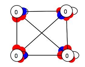
If you put this network in some initial state it may flicker around for a while before "settling down." And it may never settle down at all. It may end up cycling through a few different states over time. Dynamical systems theory gives us a vocabulary for describing these different behaviors.
To clarify these ideas, let us consider some (informally defined) concepts from dynamical systems theory. We begin with the concept of an initial condition, which is just a point in state space which we assume our system begins in.
Initial Condition: the state a system begins in.
For neural networks, this is a specification of values for its nodes. When we set the neurons at some level of activation we are setting the network in an initial condition. Often we arbitrarily choose the initial condition. In Simbrain we do this by selecting all the nodes of a network and then pressing the random button. If we repeatedly press the random button we end up putting the network in a whole bunch of initial conditions.
Dynamical system: A rule which tells us what state a system will be in at any future time, given any initial condition.
A dynamical system can be thought of visually as a recipe for saying, given any point in state space, what points the system will go to at all future times given that it started there: if the system begins here at this point at noon on Thursday, it will be at this other point at 5pm on Friday. And we can do this no matter what initial condition we find our system in. Thus dynamical systems are deterministic, they allow us to completely predict the future based on the present.
The pendulum provides a classical example of a dynamical system: if you start the pendulum off in some beginning state, we can say exactly how it will swing forever in to the future, at least in principle. Most neural networks are also dynamical systems. If you start the neural network off in some state--if you specify values for all its nodes--then based on its update rules and the way it is wired together we can say for all future times how it will behave. Thus, "running" a neural network, in Simbrain by pressing the step or the play button, corresponds to applying the dynamical rule that corresponds to it. A neural network which is predictable in this way is a dynamical system. Can you think of ways to make a neural network not be a dynamical system? We will discuss this below.
Orbit: the set of states that are visited by a dynamical system relative to an initial condition.
So, we put the neural network in some initial state, and then we run the network. It changes state as a result. Each time the neural network changes state we have a new point in activation space. If we look at all the states that result from an initial condition we get an orbit. An orbit describes one of the possible behaviors of a dynamical system over time. You put it in some starting state, and then, since it is a deterministic system, its future is set. The initial condition together with its future states is an orbit.
Invariant set: a collection of orbits.
An invariant set is just a collection of orbits, and it is "invariant" in that if a system begins somewhere in an invariant set, it will stay in that set for all time. The concept of an invariant set allows us to introduce some new concepts which are useful for understanding the different behaviors of a dynamical system.
There are at least two different ways we can classify invariant sets. First, we can classify them by their "topology" or shape. There are two especially interesting shapes for invariant sets:
Fixed point: a state that goes to itself under a dynamical system. The system "stays" in this state forever.
Periodic Orbit: a set of points that the dynamical system visits repeatedly and in the same order. The system cycles through these states over and over. The number of states in a periodic orbit is its "period." These are also known as limit cycles (when they are continuous curves).
Fixed points and periodic orbits are two particular shapes that invariant sets have. Fixed points are single points. Periodic orbits are repeating loops. Note that there are other shapes for invariant sets. For example, some really interesting invariant sets are "chaotic" or "quasi-periodic," but we will not deal with these here.
We can count how many points there are in a periodic orbit, and that corresponds to the "period" of the periodic orbit. For example, a period-2 periodic orbit consists of two points that a neural network cycles through over and over again. A period 3 periodic orbit consists of three points it cycles through, etc. Don't confuse the period of a periodic orbit with the number of periodic orbits a system has. For example, a system might have four periodic orbits, one of period 2, and three of period 3.
Another way we can classify invariant sets is according to the way states nearby the invariant set behave. Sometimes states near an invariant set will tend to go to that set. The invariant set "pulls in" nearby points. These are the stable states, the ones we are likely to see. Other times states near an invariant set will tend to go away from it. These are the unstable states, the ones we are unlikely to see.
Attractor: a state or set of states A with the property that if you are in a nearby state the system will always go towards A.
Fixed points and periodic orbits can both be attractors . These are the states of a system you will tend to observe. These are also known as equilibria.
Repellor: a state or set of states R with the property that if you are in a nearby state the system will always go away from R.
Fixed points and periodic orbits can both be repellors. You are not likely to see these in practice.
One way to think about attractors and repellors is in terms of the possible states of a penny. When the penny is lying on one face or the other, it is in an attractor, a stable fixed point: if you perturb it a little it just falls back to the same place. If you balance the penny on its edge, however, it is on a repelling fixed point. If you perturb it a little in these states it will not go back to the edge-state, but will fall over.
In the chart below, the columns correspond to different topologies or shapes that a invariant set can have. The rows corresponds to the behavior of nearby states.
|
Fixed Point |
Periodic orbit |
Other |
|
|
Attractor |
attracting fixed point |
attracting periodic orbit |
chaotic attractor, quasi-periodic attractor |
|
Repellor |
repelling fixed point |
repelling periodic orbit |
|
|
Other |
centers, saddle nodes |
The items in bold are the ones we have discussed thus far.
Activity
Make a network with four nodes, fully interconnected. To do this:
-
Create four nodes by clicking the new neuron button four times.
-
Connect the four nodes to themselves and the other four nodes. Do this by (1) selecting all the nodes and (2) right click on a target node and selecting connect. Repeat the process for each successive target node.
-
Randomize the weights by selecting all weights using "W" (or Edit > Select > Select All Weights), and either pressing the randomize button or pressing "R"
Now look for attractors and limit cycles. You do this by
-
Selecting all neurons using the keyboard command "N"
-
Randomizing these neurons by pressing pressing the randomize button or using keyboard command "R"
-
Iterating the network. Repeatedly iterate until you see a repeating pattern. The number of states it takes to go from a network state back to the same state gives you the period of an attracting periodic orbit.
Be sure to check for the zero vector! You do this by selecting all neurons and pressing "C" or the clear button.
Throughout this process it can be helpful to have a gauge open. To reset the gauge select all four neurons, right click on one of the neurons, and select set Gauge and the gauge you opened.
Perceptual reversals are a form of visual perception in which, though the total input to the retina remains constant, the perception of that input varies over time. Such phenomena have been recognized for hundreds of years, but have been of particular interest to scientists recently, as a way of studying the neural correlates of consciousness. The reason is that one can use these reversals to distinguish the neurons which code for the stimulus from those which code for the changing percept.
We will look at a neural network model of this process which employs two principles we have seen in other lessons: a winner-take-all competitive structure, and adaptation. Although the model is not directly based on biological data, it does use a neurally inspired architecture. The model is from Hugh Wilson (1999) .
We will consider two special cases of perceptual reversal: ambiguous figures and binocular rivalry.
Ambiguous figures are stimuli which the visual system can interpret in more than one way. Prolonged exposure to such a stimulus can result in an oscillation between these competing interpretations. The most famous example of an ambiguous figure is the Necker cube:
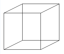
To experience the perceptual reversal fixate on this stimulus. Assuming you can see the two percepts at all, they will begin to oscillate. You will see one, then the other percept over time. Try to estimate the frequency of oscillation. Does it change roughly every 1/2 second, 1 second, 2 seconds?
Another form of perceptual reversal is observed in binocular rivalry. Whereas ambiguous figures correspond to the same image being presented to both eyes, with binocular rivalry a different image is presented to each eye. The conflict here is between these two retinal images. The visual system tries to combine them but they typically conflict in some way, resulting in a perceptual oscillation. Here is a sample stimulus:
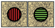
Blake and Logothetis (2002) : Visual Competition. Licensed Under OUP Licence
To get the effect you will need to create a septum (a separation between your eyes), so that each image goes to one eye only. You can do this by printing the image, placing an envelope or piece of cardboard between the images, and placing your nose directly over the envelope. You have to sort of unfocus to get the two images to line up. When they do, you should observe an oscillation between the images, as well as moments when the two images merge into a kind of patchwork. Again try to estimate the frequency of oscillation.
The neural network model of perceptual reversal is contained in networks > firingRate > perceptualReversal.net. Feel free to open it now. It is based on a model by Hugh Wilson (1999, pp. 131-134) . The model has the architecture below:
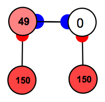
The input neurons, which are clamped, correspond to a stimulus. The output neurons correspond to two possible perceptual interpretations. Note that they are connected by inhibitory neurons and so will end up competing. The basic idea is that we are modeling input channels which feed to competing neural structures. Don't let the identical rates of firing of the inputs fool you. In the case of binocular rivalry, we can just assume that the two inputs code for different patterns, (e.g. left bars and upward bars) both of which are strongly activated.
These are Naka Rushton firing rate models with spike frequency adaptation, so the numbers are supposed to correspond to number of spikes per second, or more generally, level of activation in a neural population. These neuron types are based on integrated differential equations, so you will see an explicit time in the time label.
To see the simulation in action, press play. You will note that the two output neurons, which correspond to the two interpretations, slowly oscillate from one interpretation to the other over time. The goal is to produce an oscillation at the output nodes which matches the frequency of a real perceptual oscillation. To time the simulation, reset the time to 0 by double clicking on the time label. Do this when one output neuron is maximal. Now run the simulation and stop it when the other output neuron is maximal. This gives the time between perceptual interpretations. Compare this with the time elapsed between the reversals when you observed the two inputs.
The mechanism works as follows. The two output neurons produce a winner take all structure, since they mutually inhibit one another. But they also have spike frequency adaptation. When the simulation begins, notice that one neuron already has an activation of 1, while the other's activation is 0. This slight bias allows that neuron to initially win the competition. However, as that neuron continues to fire, adaptation kicks in, and it reduces its activity, which in turn allows the other neuron to win the competition. But then its adaptation begins to kick in, and the reverse process occurs.
To change the frequency of perceptual reversal change the firing rate time constants at the output nodes (select them both and double click to change their parameters), and modify the time step accordingly (as you make the time constants smaller, and thereby increase the time it takes for perceptual reversals to occur, you will also have to lower the time step of integration to avoid numerical errors).
To visualize these dynamics try opening a gauge and setting it to gauge the two output nodes. I recommend you set the point size (in preferences > graphics preferences) to .8, and "only add new points if this far from any other point" to .8 (in preferences > general preferences) in the gauge.
You will observe a limit cycle with a figure-8 shape, which looks like this:
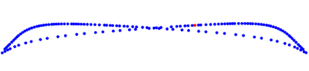
The two ends correspond to the two perceptual interpretations. Notice that the system spends a longer time on the edges of the cycle, which correspond to the different interpretations, than in the transitional portion of the figure in the middle.
Blake R and Logothetis N (2002). Visual competition. Nature Reviews Neuroscience, 3, 1 - 11.
Braitenberg, V (1984). Vehicles: Experiments in Synthetic Psychology. Cambridge, MA: MIT Press.
Churchland P (1986). Some Reductive Strategies in Cognitive Neurobiology. Mind 95:279-309.
Clark A and Chalmers D (1998). The Extended Mind. Analysis. 58:1, pp. 7-19.
Dayan P and Abbott LF (2001). Theoretical Neuroscience: Computational and Mathematical Modeling of Neural Systems. Cambridge, MA: MIT Press.
Hotton S and Yoshimi J (In Preparation). Neural Networks as Open Systems.
Hopfield J (1984). Neurons with graded response have collective computational properties like those of two-state neurons. Proceedings of the National Acadamy of Science 81:10. pp. 3088-3092.
Laurent G (1999). A Systems Perspective on Early Olfactory Coding. Science 22. Vol. 286. no. 5440, pp. 723 - 728.
Izhikevich E (2004). Which Model to Use for Cortical Spiking Neurons? IEEE Transactions On Neural Networks, Vol. 15, No. 5, pp. 1063-1070.
Sammon J (1969). A Non-linear Mapping for Data Structure Analysis. IEEE Transactions on Computers C-18: 401-409.
Wilson H (1999). Spikes, Decisions, and Actions. Oxford: Oxford University Press.
License
Any party may pass on this Work by electronic means and make it available for download under the terms and conditions of the Digital Peer Publishing License. The text of the license may be accessed and retrieved via Internet at http://www.dipp.nrw.de/lizenzen/dppl/dppl/DPPL_v2_en_06-2004.html