
Document Actions
ModelDB in Computational Neuroscience Education
A research tool as interactive educational media
Neurobiology Department, Yale University School of Medicine, 333 Cedar Street, New Haven, USA, Phone: +(USA) 203-785-5843, Fax: +(USA) 203-785-6990 email: Tom.Morse@yale.eduurn:nbn:de:0009-3-14092
Abstract. ModelDB's mission is to link computational models and publications, supporting the field of computational neuroscience (CNS) by making model source code readily available. It is continually expanding, and currently contains source code for more than 300 models that cover more than 41 topics. Investigators, educators, and students can use it to obtain working models that reproduce published results and can be modified to test for new domains of applicability. Users can browse ModelDB to survey the field of computational neuroscience, or pursue more focused explorations of specific topics. Here we describe tutorials and initial experiences with ModelDB as an interactive educational tool.
Keywords: Neuronal networks, neuronal model, biologically realistic, ion channel, kinetics, electrical excitability

ModelDB (Figure 1) is a database of computational models that has been under development for more than a decade ( Peterson et al. 1996 , Migliore et al. 2003 , Hines et al. 2004 ) as part of the SenseLab collection of Neuronal and Olfactory databases. As of August 21, 2007 it contained 312 models, and the number of model entries is currently growing at a rate of about 50 per year.
Figure 1: ModelDB home page http://senselab.med.yale.edu/modeldb
Its primary purpose is to support the field of computational neuroscience by facilitating the sharing of model code, i.e. computer programs that simulate the operation of biological neural systems. The benefits of model sharing have been reported elsewhere (see Morse 2007 for references); here we discuss and demonstrate ModelDB's supportive role in computational neuroscience education.
Although ModelDB has obvious utility in CNS research, it is also quite useful as an educational tool, because it offers the opportunity for surveying the field of CNS and also for focused study of specialized areas. An overview of CNS is possible because the hundreds of models in ModelDB begin to statistically sample the field, with an admitted bias toward "author-volunteered models" (models voluntarily contributed by their authors) and "high interest models" (models reproduced from publications by implementors other than the original model authors). Focused learning in selected topics is also possible because some research areas are well represented by models in ModelDB. Below we describe ModelDB, review CNS fields represented in ModelDB, indicate it's educational settings, present example tutorials, and describe initial experiences with ModelDB in education.
The essential data (primary attribute) of each model in ModelDB is model code, which means computer programs or specifications in XML that are automatically convertible to computer programs. Citations of papers that introduce, develop, or use the model are attached to each model entry. These provide the scientific context of the model and permit the model to be found with searches by author.
Keywords can also be attached to models. Keywords are listed on the ModelDB home page and in lists of keywords-pages linked from the ModelDB home page. Clicking on a keyword displays all the names of models to which that keyword is attached. Each model name links to a page from which the model code may be downloaded and which shows all the papers and keywords associated with that model.
Keywords include many different cell names (i.e. clicking on "Cell Type" (figure 1) leads to figure 2), ion channels (currents), receptors, and also (currently) 27 simulators and simulation environments. ModelDB contains models from simulators mentioned in this volume [1]. For computational neuroscience subfields, "Topic" categories identify broad fields that models might fall under, for example diseases, or patterns of activity in neurons or networks such as oscillations, bursting, or synchronization. There is a "Tutorial/Teaching" topic keyword which currently lists ten models that were either developed from the outset for educational use or have been used as teaching material by the model submitter.
Summary of population of models in ModelDB: At present there are 62 network models and 125 single cell models. Many of these contain one or more ion channel models that can be used independently. In addition, the "Ion Channels" link on ModelDB's home page brings up 31 models whose largest spatial scale is the ion channel. All ion channel models can be found through the keywords page devoted to "currents", e.g. there are 72 models containing A-type potassium currents, 34 models containing T-type calcium currents, 57 containing calcium sensitive potassium currents, etc.
Applications of the 3 most prevalent classes of ModelDB models:
a) Single ion channel/receptor and kinetic models can be compared against single channel recordings and reused as building blocks in single cell and network models.
b) A single cell model is typically either for comparison's with electrophysiology experiments on single cells or for use in neural network modeling. The single cell models extend our knowledge by suggesting new experiments which refine our understanding. Their functional characteristics can indicate what a (further simplified) neuron model for network models must be able to reproduce.
c) Network models contain simplified neurons that have just enough complexity to capture the relevant dynamical behavior as experimentally measured while also being computationally inexpensive. Applications of network models range from generating activity patterns as found in healthy individuals (basic science) to, for example, tremors and seizures in Parkinson's and epilepsy, respectively (see Pathophysiology under the topics link from the ModelDB home page for a complete list).
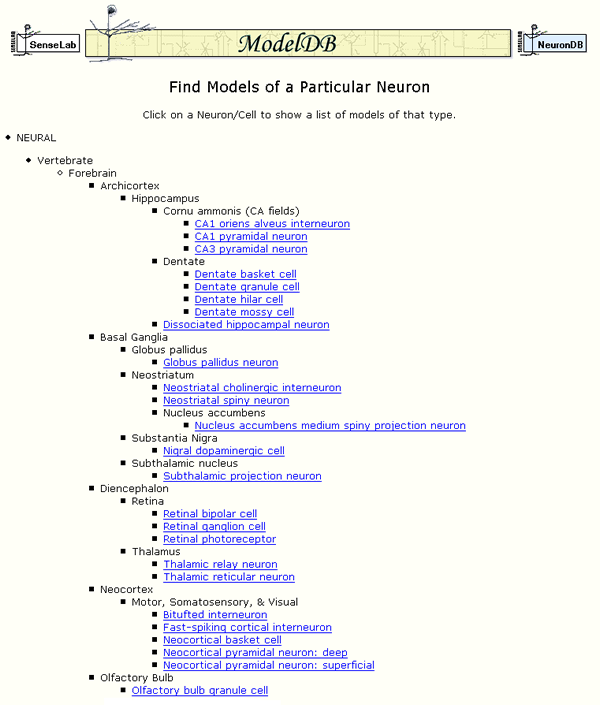
Figure 2: An excerpt from a page listing cell types for which models are available.
Potential educational users of ModelDB include advanced undergraduates, graduate and postdoctoral students, and senior investigators. The setting can be quite varied, ranging from self-study and homework problems at one extreme, to computer laboratory classroom tutorials and lecture demonstrations at the other. ModelDB can reliably provide live internet demonstrations, but it is always recomended to have models and web pages stored locally in case the internet connection goes down. See the Experience section below for an undergraduate final-exam use of ModelDB.
Before we examine specific models in ModelDB, we point out that computational models have been quite simple, of course, by comparison to real neural cells and circuits for at least four reasons. First, although much progress is being made in the way of experimental characterization of the anatomical and biophysical properties of numerous circuits and their constituent cells, many knowledge gaps still remain. Such gaps can often be filled in by informed guesses, but it is unwise to engage in wholesale speculation. A frequently occurring example of a well informed guess is that the distribution of ion channels in a cell is well represented by a constant density of numbers of these channels per area of cell membrane (for some channels where there is evidence to the contrary, a representation of the observed non-constant distribution is typically used in the model (see last tutorial)). Second, real neurons and biological networks are tremendously complex, and it is very difficult to gain a detailed understanding of the main aspects of a complex system at once. Insights must instead be teased out through the scientific method; a cycle of hypothesis formulation, testing, and revision; simplification is an essential first step in this process. Usually prior research focused on a particular aspect of neural function well enough that a clear hypothesis as to which anatomical and biophysical properties essential for it can be stated. Third, in some cases it is possible to express a hypothesis in a highly "reduced" mathematical form tractable to a combination of numerical simulation and dynamical system analysis. This approach has lead to wide-reaching theoretical insights (for examples, see the work of Varela et al. 1997 , Kopell et al. 2000 , Golomb et al. 1994 ). Fourth, network and optimization models must be simple enough that they are not to computationally expensive (not to demanding of computer memory so that they fit on available computers, and not taking to long to run so they may be productively used). Example simplifications include reducing the number of neurons (therefore also reducing the number of connections), reducing the number of compartments in a cell morphology (for networks or single cell optimizations), and substituting a simpler ion channel model for a more complex one (for single cell optimizations).
Tutorial Prerequisites: A familiarity with the Hodgkin-Huxley model ( Hodgkin and Huxley 1952 ) and electrotonic cable properties provides the required background. The tutorial models contain additional voltage gated ion channels whose mathematical details are not presented here (these additional channels are well presented in textbooks, for example Johnston and Wu 1997 , Bower and Beeman 1998 ). A numerical experimentation approach in the below tutorials facilitates undergraduate-level access to advanced research topics.
Goals: Scientific goals of the tutorial are to teach the definitions of the word "burst" and to provide familiarity with distributions of the active conductances and electrical activity over the cell's extended shape (note the later are not possible to represent in single compartment models). A technical goal is to give the student familarity with the NEURON simulator to explore NEURON models.
Part 1: We review the definition of bursting and run the CA3 Pyramidal Neuron model by Migliore et al 1995 (described below) with the NEURON simulator ( Hines and Carnevale 1997 , 2000 ):
http://senselab.med.yale.edu/ModelDB/ShowModel.asp?model=3263
Definitions and characteristics of a burst: the most commonly accepted definition of a burst is two or more spikes followed by a period of quiet ( Izhikevich 2006 ). This is consistent with early experimental papers on bursts (for example Schwartzkroin 1975 defines bursts as simply multiple discharges). The reader should be cautioned that an alternative definition exists; many experimentalists define a burst to be a sustained depolarization with spikes superimposed on top of that. Some experimentalists even classify the depolarization without multiple spikes as a burst because if the membrane was depolarized a little more, or if Na channels were not as blocked or rundown etc., there would have been APs superimposed with the depolarization (see for example figure 1C in Liu et al. 1998 ). In most cases the two definitions agree.
The paper's ( Migliore et al. 1995 ) model was used by the authors to test several hypotheses and make predictions. They incorporated known channels into a model with a realistic morphology to produce firing patterns and calcium distributions that could be compared to previous and future experiments.
This paper ( Migliore et al. 1995 ) built on at least 5 previous CA3 model papers which could reproduce some features of CA3 neurons; none of these previous papers could reproduce certain experimental results that have important functional consequences. The limits on experimental knowledge of channel densities make modeling challenging. Conductances are set according to experimental knowledge when available, otherwise modelers set the remaining conductances by optimization or by hand by trial and error to produce a neuron with desired responses to stimulation or spontaneous activity patterns. The authors discuss this mentioning that the solution space (distributions of channels that may work equally well) is potentially very large. Figures 3, 6, 7, 8 from Migliore et al. 1995 illustrate experimental spike trains that the model can match.
The notes supplied to describe the model in ModelDB state how the model "Demonstrates how the same cell could be bursting or non bursting according to the Ca-independent conductance densities. Includes calculation of intracellular Calcium". We will now run the model to examine these.
Auto-launch the model and press the "run burst" button. Traces similar to those in Figure 3 should appear.
Use the cross-hair feature by clicking on the trace in between the action potentials to verify that the membrane voltage falls to around -50 mV between the spikes during the burst.
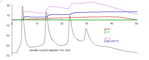
Figure 3: Migliore et al. 's 1995 CA3 model producing a burst. Note that between the APs the cell is depolarized to around -50 mV.
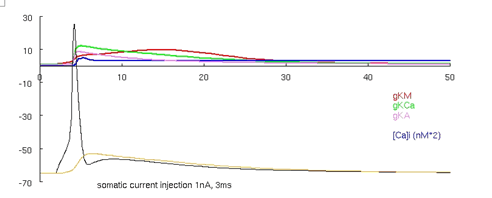
Figure 4. Migliore et al.'s 1995 CA3 model producing an AP.
Now run the model again by pressing the "run no-burst short" button. This runs the model with increased voltage gated potassium current conductances and with the same current stimulus. The simulation should produce the traces visible in Figure 4 (an animated ca3_1995.gif is also available in the supplemental material - see discussion later). These two versions of the model are created by constant conductance values distributed across the neuron taken from one of two parameter sets (the third run button below the graph runs the same model as the second button, at a reduced current injection). Keep this in mind for comparison to other cortical neuron models shown in the next and the last tutorials, where conductance values vary over the spatial extent of the neuron (rather than being constant). See Migliore et al. 1995 for more details about bursts and CA3 cell features.
As an aside, we introduce "Model View", a powerful NEURON tool that enables modelers to see the values of the parameters of the model while the model is running. This is very helpful because parameters are frequently changed in multiple places in CNS simulation code making it difficult to know what each parameter is set to at run time. For parameters that change over the spatial extent of the neuron, Model View will generate insightful parameter versus distance graphs.
Select from the NEURON main menu: Tools -> Model View. Open the "1 real cells", "root soma", and then "16 inserted mechanisms" by successively double clicking on them; the run-time values for the conductances are displayed (Figure 4). If the model is run again, after changes are made to the model, then Model View needs to be restarted so that it is refreshed.
As an example, examine the parameter, gkdrbar_borgkdr, the conductance value of the potassium delayed rectifier current, which is set to 0.03 (S/cm2) (figure 4). If the first run button is pressed again ("run burst") then the value changes back to 0.009 (S/cm2) (visible after Model View is restarted to be refreshed).
These conductance values are also visible from the NEURON main menu by selecting Tools -> Distributed Mechanisms -> Viewers ->Name Values, and then double clicking on a compartment.
Although this later method of displaying single compartment values is refreshed automatically when the model changes, Model View has the advantage that it computes all the combinations that parameters occur in, and lets you view these unique subsets of parameters that are distributed across the neuron. It is the extra computation of figuring out the unique subsets of parameters that exist in the model, that require Model View to be restarted when the model changes.
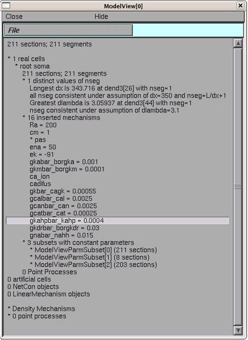
Figure 5: Run-time values of model parameters displayed in Model View.
Part 2: CA3 pyramidal neuron from Lazarewicz et al 2002 .
The model shows how using a CA1-like distribution of active dendritic conductances in a CA3 morphology results in dendritic initiation of spikes, and interacting electrical activity in the spatial extent of the cell during a burst.
This model is an updated version of the Migliore et al 1995 model incorporating new experimental information on the distribution of active conductances. A brief current pulse to the soma (see the supplemental movie CA3_2002.gif) elicits the initial soma spike which is then followed by a spike initiated in the dendrites. Then a complex interaction ensues with regenerative action potentials in the basal and apical dendrites triggering and being triggered by action potentials in the soma. The pattern of the membrane voltage activity is reminiscent of water waves. The new channel distributions in this model produces a burst pattern at the soma similar to the 1995 model, each of which is similar to those recorded experimentally at the soma. The recording of the burst at the (model) soma (see supplemental figure CA3_2002.gif) gives no hint of the electrical signals propagating throughout the spatial extent of the (model) cell. In contrast the previous 1995 model's dendrites follow the soma voltage without the dendrites regenerating spikes in the soma (see animation in supplemental material ca3_1995.gif). Future experiments with voltage or calcium activated dyes might lend support to either or possibly both models descriptions of the electrical behaviors of CA3 neurons.
Goals: The goal of this tutorial is to understand that the shape of the neuron contributes to its firing patterns (an earlier view was that the intrinsic currents formed the firing patterns). More advanced students can explore the reduced two compartment model to understand how.
We will explore the Mainen and Sejnowski 1996 models (described below):
http://senselab.med.yale.edu/ModelDB/ShowModel.asp?model=2488
Running the NEURON simulation demonstrates that an entire spectrum of firing patterns can be reproduced in this set of model neurons which share a common distribution of ion channels and differ only in their dendritic geometry, thus highlighting the importance of morphological contributions to cell electrical behavior. The zip archive contains compartmental models of four reconstructed neocortical neurons (layer 3 Aspiny, layer 4 Stellate, layer 3 and layer 5 Pyramidal neurons) with active dendritic currents.
The authors describe the common distribution of channels as follows: "This model included a low density of Na channels in the soma and dendrites and a high density in the axon hillock and initial segment. Fast K channels were present in the axon and soma but excluded from the dendrites".
Run the model by auto-launching it from ModelDB, or following the instructions in the readme.txt to run it on your platform. We will compare the layer 3 and layer 5 pyramidal cell firing patterns. Press the "L3 Pyramid" button to load that cell into the simulation. Turn on the variable time step method by selecting Tools -> VariableStepControl from the NEURON main menu, and then clicking the "Use variable dt" box. Finally press the "Init & Run" button. Preserve the graph of the membrane voltage trajectory by right-clicking on that graph and dragging the mouse (keeping the right mouse button down) to "Keep Lines" and release the mouse. When you right-click on the graph (hold right button down momentarily and release without selecting anything) now observe the "Keep Lines" menu item should have a red check mark next to it. For comparison press the "L5 pyramid" and press "Init & Run". These runs are reproducing figures 1c, 1d from Mainen and Sejnowski 1996 . What kind of firing pattern is in the last image (hint: see first tutorial)?
Note: the common distribution of ion channels is a non-uniform distribution where the axons in these models contain high Na and K channel densities at the nodes of Ranvier and the mylenated sections have low capacitance.
The authors found they could reproduce the same behavior with a two compartment model developed earlier ( Pinsky and Rinzel 1994 ). The simplified model depends on parameters rho, a ratio of dendrite membrane area to a combined soma axon membrane area, and kappa, the resistance between dendrite and combined soma axon compartments. They demonstrated the ability to reproduce each morphologically realistic model's firing patterns with the simplified model and developed insight into the relationship between the rho and kappa parameters of the reduced model and the amounts of dendritic membrane area and dendritic membrane electrical distance from the soma. (see Figures 2-4 in their paper).
The relative times of arrival and spatial positions of coincident synaptic inputs effect on the soma voltage is additionally modulated by intrinsic currents
This tutorial on the modulation of temporal integration windows is based on parts of Migliore and Shepherd 2002 (described below):
http://senselab.med.yale.edu/modeldb/ShowModel.asp?model=7659
Since electrical models of cells include the densities and kinetics of channels the importance of experimental knowledge for channels within all modeled cell types can not be overstated. The authors review the experimental knowledge of distributions of active channels on dendrites. They then discuss insights into the computational role of these channels.
Figure 2 in Migliore and Shepherd 2002 shows experimentally measured cellular Na, KA, H and Ca channel conductance distributions. There are many constant densities (17) and occasionally rising and falling conductances (11) as a function of spatial position. In some cases there are controversies, e.g. in mitral cell lateral dendrites some investigators experiments provide supporting evidence for constant Na channels conductances while others are consistent with a drop in Na channel density as a function of distance from the soma (see p. 155 in Waters et al. 2005 and references therein). Early single cell models (before 1995) had constant maximum conductances in dendrites however since then a number of models have appeared with heterogeneous channel densities in dendrites, where respective conductances either rise or fall as a function of the distance from the soma, reflecting experimental knowledge.
This model is setup to recreate parts of figure 1 and 3 from Migliore and Shepherd 2002 , which in part, compare the peak depolarization at the soma when pairs of synapses provide inputs in the following configurations: 1) both proximal to the soma, 2) one synapse proximal, and the other, distal, 3) both distal to the soma, and 4) the same as 2, however with H current added. Run the model and try each of the four buttons in the figure to examine these cases (figure 5). Notice how the presence of the H current sharpens the coincidence detection window, with a shorter difference in synaptic time differences that would cause a spike (for an arbitrary spike threshold chosen between the resting and the peak voltages), between the red curve and the green curve.
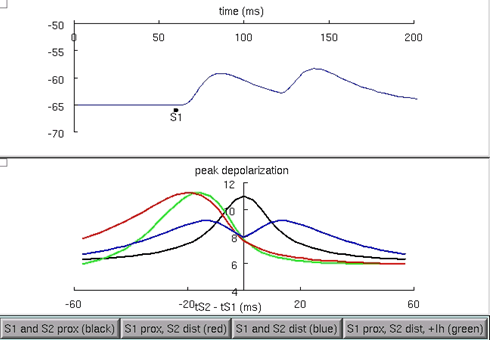
Figure 6: Comparison of the peak voltage generated at the soma from different configurations of pairs of synaptic input. When the H current is added, the peak voltage curve is sharpened from the red curve to the green curve.
Tutorial students will now demonstrate using Model View to view conductances that are a function of distance. When present, experimentally measured H conductances increase as a function of distance from the soma, i.e. see Migliore and Shepherd 2002 figure 2c). Press the lower right button (to make sure Ih is included) in the graph. Then open Model View again and view the heterogeneous densities. When you then click on "ghdbar_hd = 25 distinct values" you should then see a graph similar to figure 6.
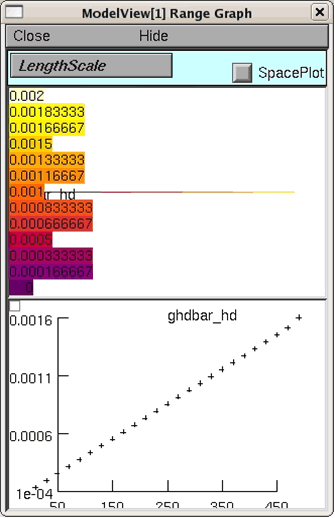
Figure 7: The increase of the H current conductance per distance from the soma displayed by Model View.
For further study:
The effects of morphology on coincidence detection and integration ( Stiefel and Sejnowski 2007 ):
http://senselab.med.yale.edu/modeldb/ShowModel.asp?model=93398
The effect of network activity on synaptic integration ( Destexhe et al. 2001 ):
http://senselab.med.yale.edu/modeldb/ShowModel.asp?model=8115
We have received a lot of positive feedback from the Computational Neuroscience community, with both professors and students finding ModelDB quite useful for teaching and research. Members of the ModelDB development team use ModelDB regularly in traditional classroom settings.
Dr. Michele Migliore, senior research scientist at the Institute of Biophysics, National Research Council, Palermo, Italy teaches Cybernetics for undergraduates in Computer Science at the University of Palermo. He uses ModelDB in his classes ( Migliore 2007 ) to discuss a few of the models at the end of the course. He asks his students to navigate it and select one of the models, according to their personal preferences, and discusses both the paper and the model during the final exam. A coefficient of difficulty (which Dr. Migliore had previously assigned to all ModelDB models) of the chosen model is considered in deciding the final score.
Dr. Ted Carnevale, senior research scientist in the Department of Neurobiology, Yale University School of Medicine, New Haven, Connecticut, recently described his experiences using ModelDB in education ( Carnevale 2007 ): "I have used ModelDB in my own teaching of neuroscience and computational modeling to undergraduates, grad students, and postdocs at Yale, and also in courses and invited seminars presented at other universities and scientific meetings. My experience has always been that students and faculty, at all levels of experience and sophistication with neuroscience and/or computational modeling, are blown away by ModelDB's contents and ease of use. I know that's slang, but it's simply the most concise way to express the effect it has on them. They are always eager to explore ModelDB on their own, and absolutely delighted, with what they find and also at the prospect of finding more of the same in the future. Many ask about how to contribute their own models that they may have developed in the past or are currently working on or planning to develop. They quickly see the value of ModelDB, not just to themselves but also to the field of computational neuroscience and the broader neuroscience community as well. In a word, the response has been not merely positive, but uniformly enthusiastic."
ModelDB is a quite useful interactive tool for students of CNS. Introductory students can gain an appreciation for and knowledge of the breadth of computational neuroscience by browsing the growing lists of topics and types of models available in ModelDB. Advanced students can benefit by interacting with computer models, gaining intuition about the effects of parameters on the behavior of systems of interest, and also can find citation information that they can refer to for further study.
The author is grateful for NIH support from grants 5P01DC004732-08 and 5R01NS011613-3, and thanks Gordon Shepherd, Ted Carnevale, and Michele Migliore for advice and proof readings, although any remaining errors are the responsibility of the author.
Av-Ron E, Byrne MJ, Byrne JH & Baxter DA (2008). SNNAP: A tool for teaching neuroscience. Brains, Minds, and Media, Vol.3, bmm1408 , this volume.
Bednar JA (2008). Understanding Neural Maps with Topographica. Brains, Minds & Media, Vol.3, bmm1402 , this volume.
Bower JM, Beeman D (1998). The book of Genesis 2nd Edition. New York Springer-Verlag.
Carnevale NT (2007). Personal communication.
Destexhe A, Rudolph M, Fellous JM, Sejnowski TJ (2001). Fluctuating synaptic conductances recreate in vivo-like activity in neocortical neurons. Neuroscience 107:13-24
Golomb D, Wang XJ, Rinzel J. (1994). Synchronization properties of spindle oscillations in a thalamic reticular nucleus model. J Neurophysiol. 72(3):1109-26.
Hines ML, Carnevale NT. 1997. The NEURON simulation environment. Neural Computation 9:1179-209.
Hines ML, Carnevale NT. 2000. Expanding NEURON's repertoire of mechanisms with NMODL. Neural Computation 12:839-51.
Hines ML, Morse T, Migliore M, Carnevale NT, Shepherd GM (2004). ModelDB: A Database to Support Computational Neuroscience. J Comput Neurosci. Jul-Aug, 17(1):7-11. Springer, Netherlends.
Hodgkin AL, Huxley AF (1952). A quantitative description of membrane current and its application to conduction and excitation in nerve. J Physiol 117:500-44
Izhikevich E (2006). Bursting, Scholarpedia p.16824 http://www.scholarpedia.org/article/Burst
Johnston D, Wu S (1997). Foundations of cellular neurophysiology. MIT Press: Cambridge.
Kopell N, Ermentrout GB, Whittington MA, Traub RD (2000). Gamma rhythms and beta rhythms have different synchronization properties. Proc Natl Acad Sci U S A. 97(4):1867-72.
Lazarewicz MT, Migliore M, Ascoli GA (2002). A new bursting model of CA3 pyramidal cell physiology suggests multiple locations for spike initiation. Biosystems 67:129-37
Liu Z, Golowasch J, Marder E, Abbott LF (1998). A model neuron with activity-dependent conductances regulated by multiple calcium sensors. J Neurosci 18:2309-20
Mainen ZF, Sejnowski TJ (1996). Influence of dendritic structure on firing pattern in model neocortical neurons. Nature 382: 363-366.
Migliore M, Cook EP, Jaffe DB, Turner DA, Johnston D (1995). Computer simulations of morphologically reconstructed CA3 hippocampal neurons. J Neurophysiol 73:1157-68
Migliore M, Morse TM, Davison AP, Marenco L, Shepherd GM, Hines ML (2003). ModelDB: making models publicly accessible to support computational neuroscience. Neuroinformatics 1(1):135-9.
Migliore M, Shepherd GM (2002). Emerging rules for the distributions of active dendritic conductances. Nature Review Neuroscience 3:362-70
Migliore M (2007). Personal communication.
Morse TM (2007). Model Sharing in Computational Neuroscience. Scholarpedia, p.15974.
Peterson BE, Healy MD, Nadkarni PM, Miller PL, Shepherd GM (1996). ModelDB: an environment for running and storing computational models and their results applied to neuroscience. J Am Med Inform Assoc. 33(6):389-98.
Pinsky PF, Rinzel J (1994). Intrinsic and network rhythmogenesis in a reduced Traub model for CA3 neurons. J Comput Neurosci 1:39-60
Schwartzkroin PA (1975). Characteristics of CA1 neurons recorded intracellularly in the hippocampal in vitro slice preparation. Brain Res. 85(3):423-36.
Stiefel KM, Sejnowski TJ (2007). Mapping Function onto Neuronal Morphology. J Neurophysiol 98:513-526
Stuart A (2008). Neurons in Action in Action - Educational settings for simulations and tutorials using NEURON. Brains, Minds & Media, Vol.3, bmm1401 , this volume.
Varela JA, Sen K, Gibson J, Fost J, Abbott LF, Nelson SB (1997). A quantitative description of short-term plasticity at excitatory synapses in layer 2/3 of rat primary visual cortex. J Neurosci 17:7926-40
Waters J, Schaefer S, Sakmann B (2005). Backpropagating action potentials in neurones: measurement, mechanisms and potential functions. Prog Biophys Mol Biol. 87(1):145-70.
[1] SNNAP ( Av-Ron et al. 2008 ), Topographica ( Bednar 2008 ), as well as models developed by collaborations which included one of the creators of Neurons in Action ( Stuart 2008 ).
License
Any party may pass on this Work by electronic means and make it available for download under the terms and conditions of the Digital Peer Publishing License. The text of the license may be accessed and retrieved via Internet at http://www.dipp.nrw.de/lizenzen/dppl/dppl/DPPL_v2_en_06-2004.html